DG Poisson

This tutorial follows python/demo/demo_dg_poisson.py. It extends the scalar cut Poisson demo to a discontinuous Galerkin space, so the physical cells, the embedded boundary, and the interior skeleton all become part of the cut integration problem. The cut DG formulation is closest to the stabilized cut discontinuous Galerkin framework cited in the related literature below.

The DG problem is solved on an unfitted circular domain; active cells and the interior skeleton are clipped by the same level set.

Model Problem

The physical domain is the negative phase of a circular level set function,

\[ \Omega=\{x\in[-1,1]^2:\phi(x)<0\},\qquad \phi(x,y)=\sqrt{(x-0.08)^2+(y+0.04)^2}-0.61 . \]

The demo solves

\[ -\Delta u=f\quad\text{in }\Omega,\qquad u=g\quad\text{on }\Gamma=\{\phi=0\}, \]

with the manufactured field

\[ u_\mathrm{ex}(x,y)=\sin(\pi x)\sin(\pi y). \]

Implementation Order

The demo runs in this order:

1. Define the circular level set.

2. Build the triangular background mesh and interpolate the P1 level set.

3. Classify inside/active/cut cells, create cell and interface runtime rules, then cut the active interior skeleton.

4. Build dx_omega, dS_omega, dx_gamma, and dS_ghost.

5. Build the DG space, SIPG volume/skeleton terms, Nitsche boundary terms, and ghost penalty.

6. Assemble, deactivate inactive dofs from the CutFEMx form active domain, and solve the serial sparse system.

7. Interpolate exact/error fields, assemble the cut-domain \(L^2\) error, print diagnostics, and write background plus cut-domain output.

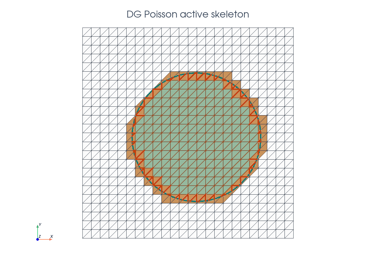
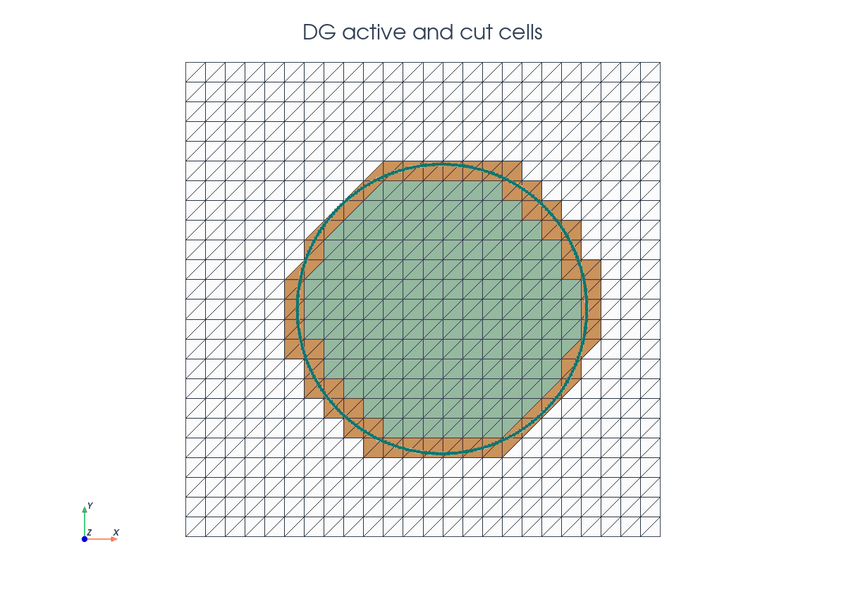
Geometry And Active Cells

The background mesh is cut once with the level set function, and predicates select the cells required by the DG formulation. Interior cells use ordinary cell integration and cut cells receive runtime quadrature rules. We also determine the active mesh formed by all interior and intersected cells. The active cell domain is used to obtain all facets that are interior to the active mesh to obtain skeleton_facets. We then compute the cut between the level set function and those facets.

Blue cells are fully inside the disk; orange cells are intersected by the embedded boundary.

cell_cut = cutfemx.cut(phi)
inside_cells = cutfemx.locate_entities(cell_cut, "phi<0")
active_cells = cutfemx.locate_entities(cell_cut, "phi<=0")
cut_cells = cutfemx.locate_entities(cell_cut, "phi=0")

skeleton_facets = cutfemx.interior_facets_for_cells(msh, active_cells)
skeleton_cut = cutfemx.cut(phi, skeleton_facets, facet_dim)

omega_interior_facets = cutfemx.locate_entities(skeleton_cut, "phi<0")
cut_skeleton_facets = cutfemx.locate_entities(skeleton_cut, "phi=0")

Runtime Quadrature

The DG form uses three kinds of cut quadrature: volume rules on \(K\cap\Omega\), interface rules on \(K\cap\Gamma\), and skeleton rules on \(F\cap\Omega\) for active interior facets.

Blue points mark cut-volume rules, magenta points mark embedded-boundary rules, and orange points mark skeleton rules on the clipped interior facets.

cell_rules = cutfemx.runtime_quadrature(cell_cut, "phi<0", order)
interface_rules = cutfemx.runtime_quadrature(cell_cut, "phi=0", order)

omega_cut_facet_rules = cutfemx.runtime_quadrature(skeleton_cut, "phi<0", order)

These rule sets define the measures used by the UFL form:

dx_omega = ufl.Measure(
    "dx", domain=msh, subdomain_id=0, subdomain_data=[inside_cells, cell_rules]
)
dx_gamma = ufl.Measure("dx", domain=msh, subdomain_id=1, subdomain_data=interface_rules)
dS_omega = ufl.Measure(
    "dS",
    domain=msh,
    subdomain_id=0,
    subdomain_data=[omega_interior_facets, omega_cut_facet_rules],
)

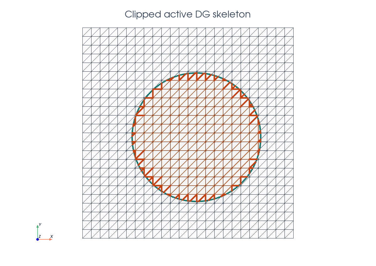
For the DG skeleton this measure has two pieces. omega_interior_facets contains the full background interior facets that lie inside \(\Omega\). omega_cut_facet_rules contains runtime quadrature on the clipped pieces \(F\cap\Omega\) for facets cut by \(\Gamma\); its parent map corresponds to the cut_skeleton_facets diagnostic set.

Active DG Skeleton

The skeleton terms are only integrated on the part of each active interior facet that belongs to \(\Omega\). Facets fully inside \(\Omega\) contribute as ordinary background facets. Intersected facets only contribute on the clipped segment \(F\cap\Omega\), so the background support facet and the integration facet are not the same geometric object.

Muted orange facets are integrated fully; gray facets are intersected support facets, and the darker orange subsegments are the clipped parts used by `dS_omega`.

With \(h\) the cell diameter and \(\sigma\) the DG penalty, the symmetric interior penalty part has the form

\[ \int_\Omega \nabla u\cdot\nabla v\,dx -\int_{\mathcal F_h^\Omega}\{\nabla u\}\cdot [v n]\,dS -\int_{\mathcal F_h^\Omega}\{\nabla v\}\cdot [u n]\,dS +\int_{\mathcal F_h^\Omega}\frac{\sigma}{h}\,[u n]\cdot[v n]\,dS . \]

n_facet = ufl.FacetNormal(msh)
h = ufl.CellDiameter(msh)
h_avg = ufl.avg(h)
sigma = penalty * degree**2

a = ufl.inner(ufl.grad(u), ufl.grad(v)) * dx_omega
jump_u = ufl.jump(u, n_facet)
jump_v = ufl.jump(v, n_facet)
a += -ufl.inner(ufl.avg(ufl.grad(u)), jump_v) * dS_omega
a += -ufl.inner(ufl.avg(ufl.grad(v)), jump_u) * dS_omega
a += sigma / h_avg * ufl.inner(jump_u, jump_v) * dS_omega

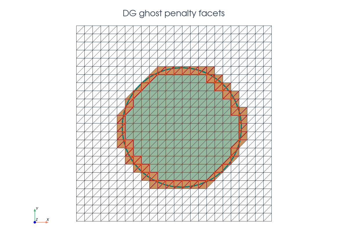
Boundary And Ghost Stabilization

The Dirichlet condition on \(\Gamma\) is imposed with Nitsche terms. A ghost penalty then couples cut cells to neighboring interior cells, reducing the conditioning sensitivity caused by very small intersections.

Red facets indicate the ghost-penalty band near the embedded boundary.

n_gamma = cutfemx.normal(phi)
ghost_facets = cutfemx.ghost_penalty_facets(cell_cut, "phi<0")
dS_ghost = ufl.Measure("dS", domain=msh, subdomain_id=2, subdomain_data=ghost_facets)

The boundary terms use the same symmetric Nitsche structure as the continuous Poisson example, but with the DG interface penalty sigma_gamma. The source term and boundary data use the manufactured exact solution.

sigma_gamma = interface_penalty * degree**2

a += (
    -ufl.dot(ufl.grad(u), n_gamma) * v
    - ufl.dot(ufl.grad(v), n_gamma) * u
    + sigma_gamma / h * u * v
) * dx_gamma

L = f * v * dx_omega
L += (
    -ufl.dot(ufl.grad(v), n_gamma) * u_exact
    + sigma_gamma / h * u_exact * v
) * dx_gamma

Ghost Penalty Implementation

The ghost penalty is assembled on the background facets returned by cutfemx.ghost_penalty_facets. These facets form a narrow band around the cut cells and couple the DG gradients across neighboring active cells. This keeps the system better conditioned when the physical domain cuts only a very small part of a background cell.

In this demo the stabilization penalizes the normal jump of the gradient:

\[ \int_{\mathcal F_\mathrm{ghost}} \gamma_g h_\mathrm{avg} [\![ \nabla u \cdot n_F ]\!] [\![ \nabla v \cdot n_F ]\!] \,dS . \]

In UFL, ufl.jump(ufl.grad(u), n_facet) represents this normal gradient jump. The term is only added when the ghost-facet set is non-empty.

if ghost_facets.size > 0:
    a += (
        ghost_penalty
        * h_avg
        * ufl.inner(
            ufl.jump(ufl.grad(u), n_facet),
            ufl.jump(ufl.grad(v), n_facet),
        )
        * dS_ghost
    )

Solver And Error

The final forms are wrapped as CutFEMx runtime forms. The assembly path builds a serial sparse MatrixCSR, scatters the contributions, deactivates degrees of freedom outside the active cut domain, and solves the resulting system with SciPy.

a_form = cutfemx.fem.form(a)
L_form = cutfemx.fem.form(L)

A = cutfemx.fem.assemble_matrix(a_form)
A.scatter_reverse()
b = cutfemx.fem.assemble_vector(L_form)
b.scatter_reverse(la.InsertMode.add)

cutfemx.fem.deactivate_outside(A, b, cutfemx.fem.active_domain(a_form))

from scipy.sparse.linalg import spsolve

uh = fem.Function(V, name="u_h")
uh.x.array[:] = spsolve(A.to_scipy().tocsr(), b.array)
uh.x.scatter_forward()

After the solve, the demo interpolates the exact field into the DG space and computes both a background error function and the cut-domain \(L^2\) error using the same dx_omega measure as the variational form.

u_exact_bg = fem.Function(V, name="u_exact")
u_exact_bg.interpolate(lambda x: np.sin(np.pi * x[0]) * np.sin(np.pi * x[1]))
u_exact_bg.x.scatter_forward()

error_bg = fem.Function(V, name="u_error")
error_bg.x.array[:] = uh.x.array - u_exact_bg.x.array
error_bg.x.scatter_forward()

error_form = cutfemx.fem.form((uh - u_exact) ** 2 * dx_omega)
error_sq = cutfemx.fem.assemble_scalar(error_form)
error_sq = comm.allreduce(error_sq, op=MPI.SUM)

Solution Output

The solution is visualized on the cut disk.

DG poisson solution on cut geometry.

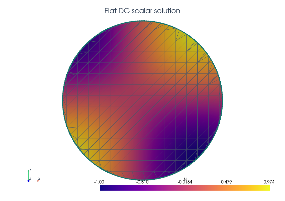
The output routine writes both the background fields and their restrictions to the physical cut domain. The cut mesh is an output mesh only.

cut_mesh = cutfemx.create_cut_mesh(cell_cut, "phi<0", mode="full")

phi_cut = cutfemx.fem.cut_function(phi_out, cut_mesh)
uh_cut = cutfemx.fem.cut_function(uh_out, cut_mesh)

cut_path = output_dir / "dg_poisson_cut_domain.xdmf"
with io.XDMFFile(comm, cut_path.as_posix(), "w") as xdmf:
    xdmf.write_mesh(cut_mesh.mesh)
    xdmf.write_function(phi_cut)
    xdmf.write_function(uh_cut)

The script writes:

• dg_poisson_xdmf/dg_poisson_background.xdmf

• dg_poisson_xdmf/dg_poisson_cut_domain.xdmf

Related Literature

• C. Gürkan and A. Massing, “A stabilized cut discontinuous Galerkin framework for elliptic boundary value and interface problems”, Computer Methods in Applied Mechanics and Engineering 348, 466-499, 2019. This paper develops the unfitted SIPG/CutDG framework for elliptic boundary-value and interface problems, including Poisson problems and ghost-penalty stabilization.

Run The Demo

python python/demo/demo_dg_poisson.py

Full Source

The complete source remains available in the repository: python/demo/demo_dg_poisson.py.