Interface Poisson

This tutorial follows python/demo/demo_interface_poisson.py and presents a multi-domain Poisson problem. The Nitsche coupling over the unfitted interface is related to the CutFEM interface literature listed in the related literature below.

Multi-domain poisson problem with contrast in diffusivities.

Model Problem

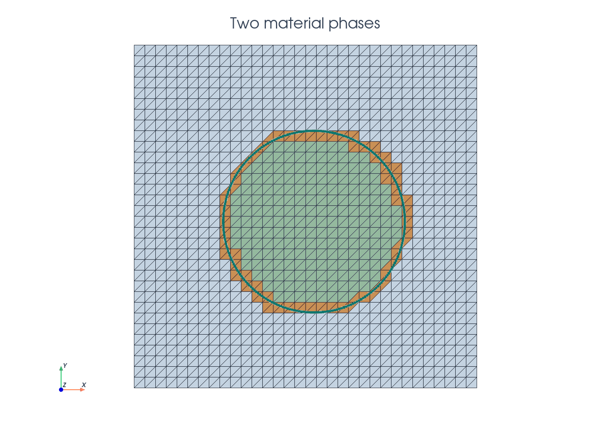
Let \(\Omega_0=[-1,1]^2\) be the background domain. A circular level set partitions this box into two material phases,

\[ \Omega_1=\{x:\phi(x)<0\},\qquad \Omega_2=\{x:\phi(x)>0\},\qquad \Gamma=\{x:\phi(x)=0\}. \]

The demo uses

\[ \phi(x,y)=\sqrt{(x-x_c)^2+(y-y_c)^2}-R, \]

with \((x_c,y_c)=(0.05,-0.03)\) and \(R=0.53\) by default. In each phase it solves

\[ -\nabla\cdot(\kappa_i\nabla u_i)=f_i \quad\text{in }\Omega_i,\qquad i=1,2, \]

with transmission conditions on the internal interface,

\[ u_1-u_2=0,\qquad \kappa_1\nabla u_1\cdot n_\Gamma -\kappa_2\nabla u_2\cdot n_\Gamma=0 \quad\text{on }\Gamma. \]

The manufactured solution is continuous and has balanced normal flux:

\[ u_1=(x-x_c)^2+(y-y_c)^2, \]

and

\[ u_2=\frac{\kappa_1}{\kappa_2} \left((x-x_c)^2+(y-y_c)^2\right) +R^2\left(1-\frac{\kappa_1}{\kappa_2}\right). \]

With these choices both right-hand sides are

\[ f_1=f_2=-4\kappa_1. \]

Implementation Order

1. Define level set function.

2. Interpolate the P1 circular level set and build cut_data.

3. Locate inside/outside cells, create phase/interface runtime quadrature, and select separate ghost-facet bands for the two phase fields.

4. Build phase, interface, ghost, and outer-boundary measures.

5. Create two scalar background spaces and a UFL MixedFunctionSpace.

6. Build manufactured fields, bulk diffusion terms, Nitsche interface coupling, ghost penalties, and the weak outer boundary condition for u2.

7. Extract UFL blocks, wrap them as CutFEMx forms, compute the two active domains, and call solve_block_system(...).

8. Assemble errors and interface jump diagnostics, optionally plot, and write <prefix>_u1.xdmf and <prefix>_u2.xdmf.

Imports

The script uses DOLFINx for the background mesh and fields, UFL for the block weak form, CutFEMx for cut classification, runtime quadrature, normals, assembly, active-domain handling, and physical cut-mesh output.

from pathlib import Path

from mpi4py import MPI

import cutfemx
import numpy as np
import ufl
from dolfinx import default_scalar_type, fem, io, la, mesh
from scipy.sparse import bmat
from scipy.sparse.linalg import spsolve

Background Mesh

The interface is not fitted to the mesh. Both phase fields are defined on the same triangular background mesh, and CutFEMx restricts each field to the physical part of the mesh through phase-dependent measures and active domains.

comm = MPI.COMM_WORLD
n = 24

msh = mesh.create_rectangle(
    comm,
    ((-1.0, -1.0), (1.0, 1.0)),
    (n, n),
    cell_type=mesh.CellType.triangle,
)
fdim = msh.topology.dim - 1
msh.topology.create_entities(fdim)
msh.topology.create_connectivity(fdim, msh.topology.dim)
exterior_facets = mesh.exterior_facet_indices(msh.topology)

Level Set Function

The level set is represented by a standard P1 function on the background mesh. The sign of this function determines the two material phases.

radius = 0.53
center = (0.05, -0.03)

V_phi = fem.functionspace(msh, ("Lagrange", 1))
phi = fem.Function(V_phi, name="phi")
phi.interpolate(
    lambda x: np.sqrt((x[0] - center[0]) ** 2
                      + (x[1] - center[1]) ** 2) - radius
)

Phase Cells

One call to cutfemx.cut builds the geometric state. The negative phase is the inside disk, the positive phase is the outside material, and "phi=0" selects the cells cut by the interface.

Green cells belong to the negative phase, blue cells belong to the positive phase, and orange cells are cut by the interface.

cut_data = cutfemx.cut(phi)
inside_cells = cutfemx.locate_entities(cut_data, "phi<0")
outside_cells = cutfemx.locate_entities(cut_data, "phi>0")

These cell lists identify ordinary uncut cells in each phase. Cut cells are handled by runtime quadrature rather than by modifying the background mesh.

Runtime Quadrature

Runtime quadrature provides physical integration points for each phase and for the interface. The phase rules integrate \(K\cap\Omega_i\) on cut cells; the interface rule integrates \(K\cap\Gamma\).

Blue and green markers are cut-volume quadrature for the two phases; magenta markers are interface quadrature points.

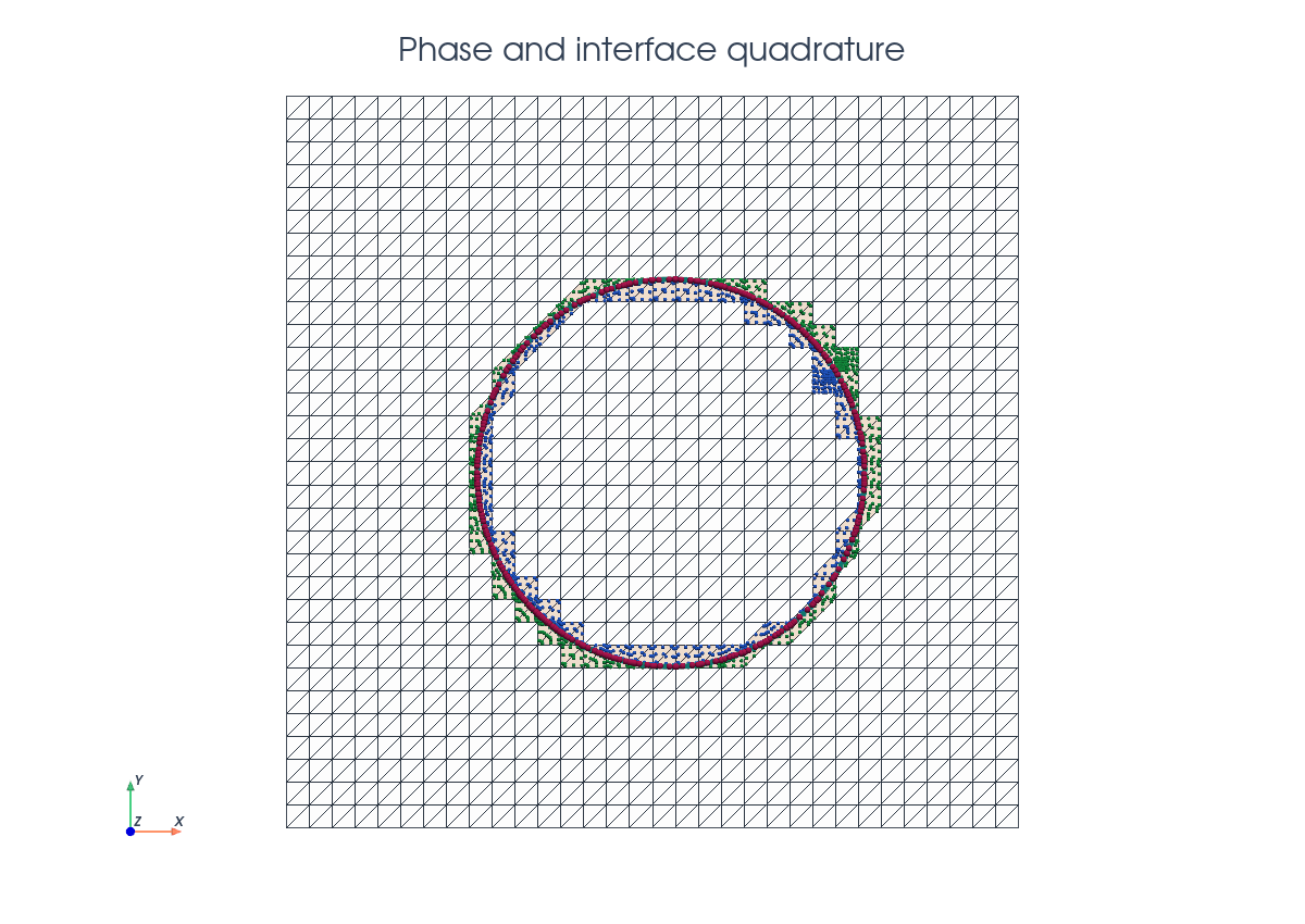
order = 4
inside_rules = cutfemx.runtime_quadrature(cut_data, "phi<0", order)
outside_rules = cutfemx.runtime_quadrature(cut_data, "phi>0", order)
interface_rules = cutfemx.runtime_quadrature(cut_data, "phi=0", order)

The standard cells and runtime rules are combined in UFL measures:

dx1 = ufl.Measure(
    "dx", domain=msh, subdomain_id=1,
    subdomain_data=[inside_cells, inside_rules],
)
dx2 = ufl.Measure(
    "dx", domain=msh, subdomain_id=2,
    subdomain_data=[outside_cells, outside_rules],
)
dgamma = ufl.Measure("dx", domain=msh, subdomain_id=3,
                     subdomain_data=interface_rules)

The interface measure is written as a UFL "dx" measure because the interface quadrature is immersed in volume cells representing a line integral over \(\Gamma\).

Phase Spaces

The two phases use separate scalar fields on the same background mesh. This is important: the traces of \(u_1\) and \(u_2\) on \(\Gamma\) are independent until the interface terms couple them.

V1 = fem.functionspace(msh, ("Lagrange", 1))
V2 = fem.functionspace(msh, ("Lagrange", 1))
W_block = ufl.MixedFunctionSpace(V1, V2)

u1, u2 = ufl.TrialFunctions(W_block)
v1, v2 = ufl.TestFunctions(W_block)

ufl.MixedFunctionSpace(V1, V2) is used here to express the coupled weak form as a two-field block problem. It does not create one physical mixed finite element field for output; instead, it gives UFL a product space with one component for the inside phase and one component for the outside phase. The trial functions u1 and u2 therefore remain associated with the separate background spaces V1 and V2, but interface terms can still contain both fields in the same expression.

This is what lets the demo write the interface coupling once as a single UFL form and then split it into the four matrix blocks

\[\begin{split} \begin{pmatrix} A_{11} & A_{12}\\ A_{21} & A_{22} \end{pmatrix} \begin{pmatrix} u_1\\ u_2 \end{pmatrix} = \begin{pmatrix} b_1\\ b_2 \end{pmatrix}. \end{split}\]

The diagonal blocks are the phase diffusion, boundary, and ghost-penalty terms. The off-diagonal blocks come only from the Nitsche interface coupling, where the jump \(u_1-u_2\) and weighted flux terms involve both phases.

Manufactured Fields

The exact fields are built from the radial coordinate around the interface center. The outside field is scaled so that the solution and the normal flux match the inside field at \(r=R\).

x = ufl.SpatialCoordinate(msh)
r2 = (x[0] - center_x) ** 2 + (x[1] - center_y) ** 2
ratio = kappa_1 / kappa_2

u1_exact = r2
u2_exact = ratio * r2 + radius**2 * (1.0 - ratio)

f1 = fem.Constant(msh, default_scalar_type(-4.0 * kappa_1))
f2 = fem.Constant(msh, default_scalar_type(-4.0 * kappa_1))

Bulk Terms

Each phase contributes an ordinary diffusion form on its own cut-domain measure. There is no direct coupling in the volume terms.

a = kappa_1 * ufl.inner(ufl.grad(u1), ufl.grad(v1)) * dx1
a += kappa_2 * ufl.inner(ufl.grad(u2), ufl.grad(v2)) * dx2

L = f1 * v1 * dx1 + f2 * v2 * dx2

Nitsche Interface Coupling

The continuity and flux-balance conditions are imposed weakly on \(\Gamma\) with a weighted symmetric Nitsche form. CutFEMx computes the interface normal from the level-set field:

n_gamma = cutfemx.normal(phi)
h = ufl.CellDiameter(msh)

kappa_h = 2.0 * kappa_1 * kappa_2 / (kappa_1 + kappa_2)
eta_interface = gamma_interface * kappa_h / h
w1 = kappa_2 / (kappa_1 + kappa_2)
w2 = kappa_1 / (kappa_1 + kappa_2)

With jump \([u]=u_1-u_2\) and weighted normal flux

\[ \{\kappa\nabla u\cdot n\}_w =w_1\kappa_1\nabla u_1\cdot n_\Gamma +w_2\kappa_2\nabla u_2\cdot n_\Gamma, \]

the interface contribution is

\[ \int_\Gamma \left( -\{\kappa\nabla u\cdot n\}_w[v] -\{\kappa\nabla v\cdot n\}_w[u] +\eta_\Gamma [u][v] \right)\,ds. \]

jump_u = u1 - u2
jump_v = v1 - v2

flux_u = w1 * kappa_1 * ufl.dot(ufl.grad(u1), n_gamma)
flux_u += w2 * kappa_2 * ufl.dot(ufl.grad(u2), n_gamma)

flux_v = w1 * kappa_1 * ufl.dot(ufl.grad(v1), n_gamma)
flux_v += w2 * kappa_2 * ufl.dot(ufl.grad(v2), n_gamma)

a += (-flux_u * jump_v - flux_v * jump_u
      + eta_interface * jump_u * jump_v) * dgamma

Ghost Penalty Facets

Both fields need their own ghost-penalty band because each field has a different active domain. The inside band stabilizes the \(u_1\) block; the outside band stabilizes the \(u_2\) block.

The red band marks the ghost-penalty facets used to stabilize the inside field $u_1$.

The blue band marks the ghost-penalty facets used to stabilize the outside field $u_2$.

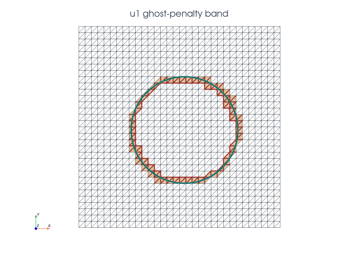
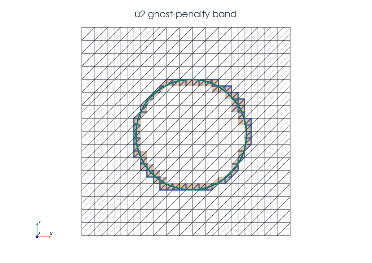
ghost_facets_1 = cutfemx.ghost_penalty_facets(cut_data, "phi<0")
ghost_facets_2 = cutfemx.ghost_penalty_facets(cut_data, "phi>0")

dS_ghost_1 = ufl.Measure("dS", domain=msh, subdomain_id=4,
                         subdomain_data=ghost_facets_1)
dS_ghost_2 = ufl.Measure("dS", domain=msh, subdomain_id=5,
                         subdomain_data=ghost_facets_2)

n_facet = ufl.FacetNormal(msh)
h_avg = ufl.avg(h)

The stabilization terms are added only when the corresponding facet set is non-empty:

if ghost_facets_1.size > 0 and gamma_ghost != 0.0:
    a += (
        gamma_ghost * kappa_1 * h_avg
        * ufl.inner(
            ufl.jump(ufl.grad(u1), n_facet),
            ufl.jump(ufl.grad(v1), n_facet),
        )
        * dS_ghost_1
    )

if ghost_facets_2.size > 0 and gamma_ghost != 0.0:
    a += (
        gamma_ghost * kappa_2 * h_avg
        * ufl.inner(
            ufl.jump(ufl.grad(u2), n_facet),
            ufl.jump(ufl.grad(v2), n_facet),
        )
        * dS_ghost_2
    )

Outer Boundary

The outside phase touches the boundary of the background box. The demo imposes the manufactured outer boundary value for \(u_2\) weakly by Nitsche terms on the exterior facets.

ds_outer = ufl.Measure("ds", domain=msh, subdomain_id=6,
                       subdomain_data=exterior_facets)
eta_boundary = gamma_boundary * kappa_2 / h

a += (
    -kappa_2 * ufl.dot(ufl.grad(u2), n_facet) * v2
    - kappa_2 * ufl.dot(ufl.grad(v2), n_facet) * u2
    + eta_boundary * u2 * v2
) * ds_outer

L += (
    -kappa_2 * ufl.dot(ufl.grad(v2), n_facet) * u2_exact
    + eta_boundary * u2_exact * v2
) * ds_outer

The inside phase does not touch the outer box boundary in this configuration, so it has no outer-boundary condition.

Block Assembly

The UFL block form is split into four matrix blocks and two right-hand-side blocks. Each block is wrapped as a CutFEMx runtime form before assembly.

a_blocks = ufl.extract_blocks(a)
L_blocks = ufl.extract_blocks(L)

a_forms = tuple(
    tuple(cutfemx.fem.form(a_blocks[i][j]) for j in range(2))
    for i in range(2)
)
L_forms = tuple(cutfemx.fem.form(L_blocks[i]) for i in range(2))

Each diagonal block carries a different active domain. After assembly, CutFEMx deactivates the inactive degrees of freedom in each block row before the two-by-two sparse block system is passed to SciPy.

domain1 = cutfemx.fem.active_domain(a_forms[0][0])
domain2 = cutfemx.fem.active_domain(a_forms[1][1])

A_matrix_blocks = [
    [_assemble_matrix_block(a_forms[i][j]) for j in range(2)]
    for i in range(2)
]
b_vector_blocks = [_assemble_vector_block(L_forms[i]) for i in range(2)]

cutfemx.fem.deactivate_outside_blocks(
    A_matrix_blocks, [domain1, domain2], b_vector_blocks
)

The demo checks that no zero rows remain after deactivation. This catches missing stabilization or active-domain mistakes before the solve.

Solve And Diagnostics

The demo assembles the serial SciPy block matrix, solves it, and scatters the two background fields.

A = bmat(
    [[A.to_scipy().tocsr() for A in row] for row in A_matrix_blocks],
    format="csr",
)
b = np.concatenate([block.array.copy() for block in b_vector_blocks])
n1 = b_vector_blocks[0].array.size

solution = spsolve(A, b)

u1_h = fem.Function(V1, name="u1_h")
u2_h = fem.Function(V2, name="u2_h")
u1_h.x.array[:] = solution[:n1]
u2_h.x.array[:] = solution[n1:]
u1_h.x.scatter_forward()
u2_h.x.scatter_forward()

After the solve, the script reports the phase-wise \(L^2\) errors and the interface jump norm:

e1 = cutfemx.fem.assemble_scalar(
    cutfemx.fem.form((u1_h - u1_exact) ** 2 * dx1)
)
e2 = cutfemx.fem.assemble_scalar(
    cutfemx.fem.form((u2_h - u2_exact) ** 2 * dx2)
)
jump_error = cutfemx.fem.assemble_scalar(
    cutfemx.fem.form((u1_h - u2_h) ** 2 * dgamma)
)

Solution Output

The final fields are written on physical cut meshes. As in the scalar cut Poisson tutorial, these meshes are visualization/output meshes only.

inside_mesh = cutfemx.create_cut_mesh(cut_data, "phi<0", mode="full")
outside_mesh = cutfemx.create_cut_mesh(cut_data, "phi>0", mode="full")

u1_cut = cutfemx.fem.cut_function(u1_h, inside_mesh)
u2_cut = cutfemx.fem.cut_function(u2_h, outside_mesh)

The script writes:

• interface_poisson_u1.xdmf

• interface_poisson_u2.xdmf

Related Literature

• E. Burman, S. Claus, P. Hansbo, M. G. Larson, and A. Massing, “CutFEM: Discretizing Geometry and Partial Differential Equations”, International Journal for Numerical Methods in Engineering 104(7), 472-501, 2015. This is the main CutFEM reference for the unfitted Nitsche formulation and ghost stabilization used in this example.

Run The Demo

python python/demo/demo_interface_poisson.py

Full Source

The complete source remains available in the repository: python/demo/demo_interface_poisson.py.