Moving Poisson

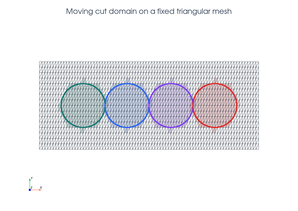
This tutorial follows python/demo/demo_moving_poisson.py. The background mesh and finite element space are fixed, while a circular level set moves through the domain. The key point is that the CutData object is created once for the reusable level-set function and then refreshed with cutfemx.update(cut_data) after the level-set coefficients change. The entity lists, runtime quadrature, ghost facets, assembled system, and cut-domain output are then rebuilt from the updated cut state. The update pattern is an implementation detail, while the underlying unfitted moving-domain formulation is related to the CutFEM references in the related literature below.

The same triangular background mesh is reused for all level-set positions.

Model Problem

At step \(k\), the physical domain is the moving disk

\[ \Omega_k=\{x:\phi_k(x)<0\},\qquad \phi_k(x,y)=\sqrt{(x-c_{k,0})^2+(y-c_{k,1})^2}-0.5 . \]

The demo solves

\[ -\Delta u_k = 1 \quad \text{in }\Omega_k, \qquad u_k=0 \quad \text{on }\Gamma_k=\{\phi_k=0\}, \]

using symmetric Nitsche terms on the embedded boundary.

Implementation Order

The demo has two implementation units. First, the top-level script creates the fixed mesh, scalar space, reusable phi function, and initial cut_data object. Then each loop iteration calls solve_step(...) followed by write_step_xdmf(...).

Inside solve_step(...) the order is:

1. Interpolate the moved circle level set into the existing phi.

2. Call cutfemx.update(cut_data) to refresh the existing cut state from the new phi coefficients.

3. Locate inside and cut cells, create runtime rules, and select ghost facets from the updated cut_data.

4. Build the Nitsche Poisson form with constant source 1 and homogeneous boundary value.

5. Assemble, deactivate inactive dofs from the CutFEMx form active domain, and solve.

6. Return the updated cut state, solution, and diagnostic entity lists to the loop.

write_step_xdmf(...) then writes the background fields and the physical cut mesh for that same step.

Fixed Mesh And Function Space

The mesh is created once on [-1,4] x [-1,1] with triangular cells. The scalar finite element space is reused for every moving-domain solve.

msh = mesh.create_rectangle(
    comm,
    ((-1.0, -1.0), (4.0, 1.0)),
    (5 * n, n),
    cell_type=mesh.CellType.triangle,
)
V = fem.functionspace(msh, ("Lagrange", 1))
phi = fem.Function(V, name="phi")
phi.interpolate(circle_level_set((0.0, 0.0), radius))
phi.x.scatter_forward()
cut_data = cutfemx.cut(phi)

The top-level loop then keeps passing that same cut_data object into solve_step(...). Inside solve_step(...), the first operation after changing phi is cutfemx.update(cut_data), so the geometry is refreshed in place before the current step is classified, assembled, solved, and written.

for step in range(steps):
    center = (float(step), 0.0)
    cut_data, uh, inside_cells, cut_cells, ghost_facets = solve_step(
        msh,
        V,
        phi,
        cut_data,
        center,
        radius,
        order,
        gamma,
        gamma_g,
    )
    uh.name = f"u_h_{step:02d}"
    write_step_xdmf(output_dir, step, cut_data, phi, uh)

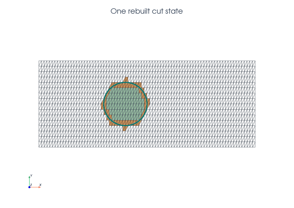
Updating One Cut State

Only the level-set coefficients and the CutFEMx geometry state change from one step to the next. The demo therefore keeps the same phi and cut_data objects and updates their contents in place.

One time step after the level set has been interpolated and the active/cut cells have been classified.

phi.interpolate(circle_level_set(center, radius))
phi.x.scatter_forward()
cutfemx.update(cut_data)

inside_cells = cutfemx.locate_entities(cut_data, "phi<0")
cut_cells = cutfemx.locate_entities(cut_data, "phi=0")

cutfemx.update(cut_data) is the operation that makes the existing geometric cut state follow the moved level set. The calls after it intentionally rebuild the step-local classifications and quadrature data from that refreshed state.

Rebuilding Quadrature And Facets

Each moved domain gets fresh runtime quadrature rules and a fresh ghost-facet set. These objects are local to the current step.

Blue and magenta points are the physical quadrature points for one moved disk.

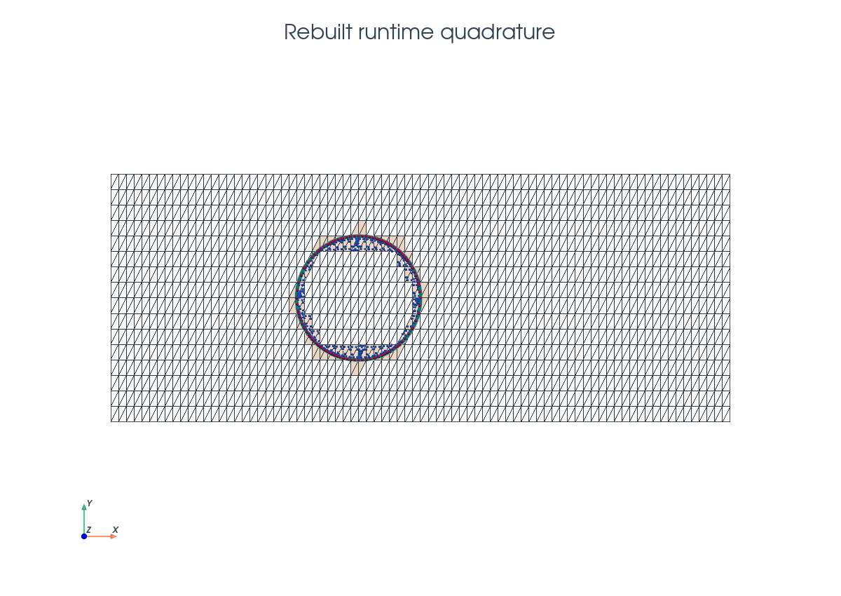
inside_rules = cutfemx.runtime_quadrature(cut_data, "phi<0", order)
interface_rules = cutfemx.runtime_quadrature(cut_data, "phi=0", order)
ghost_facets = cutfemx.ghost_penalty_facets(cut_data, "phi<0")

Per-Step Solve Algorithm

The weak form is the same Nitsche formulation as the scalar Poisson tutorial, but with a constant source and homogeneous boundary value.

Output

The output is written per step. The animation below shows the same incremental sequence: update the existing cut state, solve the current step, write that step, and then move to the next level-set position.

The cut domain is solved and visualized one updated level-set position at a time.

The script writes one background file and one cut-domain file per step in moving_poisson_xdmf/.

Related Literature

• E. Burman, S. Claus, P. Hansbo, M. G. Larson, and A. Massing, “CutFEM: Discretizing Geometry and Partial Differential Equations”, International Journal for Numerical Methods in Engineering 104(7), 472-501, 2015. This is the general CutFEM reference for fixed-background meshes, weak boundary imposition, and ghost stabilization.

• S. Claus, S. Bigot, and P. Kerfriden, “CutFEM Method for Stefan–Signorini Problems with Application in Pulsed Laser Ablation”, SIAM Journal on Scientific Computing 40(5), B1444-B1469, 2018. This gives an example of CutFEM on moving level-set-defined domains without remeshing.

Run The Demo

python python/demo/demo_moving_poisson.py

Full Source

The complete source remains available in the repository: python/demo/demo_moving_poisson.py.