Cut Poisson

This tutorial follows python/demo/demo_poisson.py. It shows how to set up a Poisson problem inside a negative level set domain. The Nitsche and ghost-penalty formulation follows the CutFEM framework summarized in the related literature below.

Scalar solution on the physical cut mesh shown with the background triangular mesh.

Model Problem

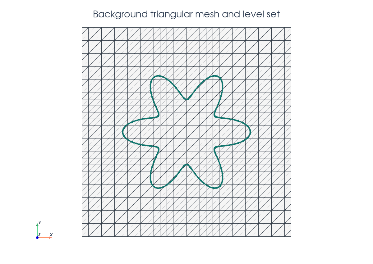
Let \(\Omega_0=[-1,1]^2\) be the background domain and let the physical domain be the negative phase of a six-petal flower level set. With \(\rho=\sqrt{x^2+y^2}\) and \(\theta=\operatorname{atan2}(y,x)\),

\[ r_\Gamma(\theta)=R_0+A\cos(m\theta), \qquad \phi(x,y)=\rho-r_\Gamma(\theta), \]

where \(R_0=0.46\), \(A=0.15\), and \(m=6\),

so that

\[ \Omega=\{(x,y)\in\Omega_0:\phi(x,y)<0\}, \qquad \Gamma=\{(x,y)\in\Omega_0:\phi(x,y)=0\}. \]

The demo solves the manufactured Dirichlet problem

\[ -\Delta u=f\quad\text{in }\Omega,\qquad u=g\quad\text{on }\Gamma, \]

with

\[ u_\mathrm{ex}(x,y)=\sin(\pi x)\sin(\pi y), \qquad f=2\pi^2u_\mathrm{ex}, \qquad g=u_\mathrm{ex}|_\Gamma . \]

Implementation Order

The script runs in this order:

1. Define the flower level set.

2. Build the triangular background mesh and interpolate the P1 level set.

3. Build cut_data, locate full inside cells, create volume/interface runtime quadrature, and select ghost-penalty facets.

4. Build the UFL measures, function space, Nitsche form, and ghost penalty.

5. Wrap the UFL forms with cutfemx.fem.form, assemble, deactivate inactive dofs using cutfemx.fem.active_domain(a_form), and solve.

6. Interpolate exact/error fields, assemble the cut-domain \(L^2\) error, print diagnostics, and write background plus cut-domain XDMF output.

Imports

The script uses DOLFINx for the mesh and function spaces, UFL for the weak form, and CutFEMx for cut classification, quadrature, normals, assembly, and cut-mesh output.

from pathlib import Path

from mpi4py import MPI

import cutfemx
import numpy as np
import ufl
from dolfinx import fem, io, la, mesh

Background Mesh

The background mesh is deliberately not fitted to the flower boundary. It is the computational mesh on which the level-set function, trial space, and assembled linear system live.

The zero level set cuts through ordinary triangular cells of the background mesh.

comm = MPI.COMM_WORLD
n = 32

msh = mesh.create_rectangle(
    comm,
    ((-1.0, -1.0), (1.0, 1.0)),
    (n, n),
    cell_type=mesh.CellType.triangle,
)

Level Set Function

The implicit geometry is represented by a standard finite element function. CutFEMx reads the level set finite element function and computes the intersection of the level set with the background mesh with cutfemx.cut. In this example, we use a linear level-set function in a triangular background mesh.

base_radius = 0.46
amplitude = 0.15
petals = 6
V_phi = fem.functionspace(msh, ("Lagrange", 1))
phi = fem.Function(V_phi, name="phi")

phi.interpolate(flower_level_set(base_radius, amplitude, petals))
phi.x.scatter_forward()

Interior Cells

Cells fully inside the negative phase use ordinary cell integration. These are the cells selected by the "phi<0" predicate.

Interior cells contribute with the usual DOLFINx cell quadrature.

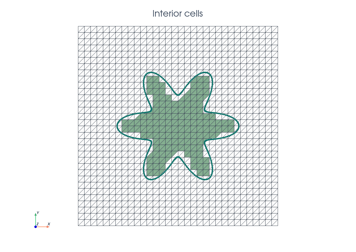
cut_data = cutfemx.cut(phi)
inside_cells = cutfemx.locate_entities(cut_data, "phi<0")

Runtime Quadrature

Cells intersected by \(\Gamma\) need to be integrated differently. The function runtime_quadrature generates runtime quadrature rules depending on how the level set intersects the cells. For the Poisson problem we need the parts of cells that intersect with the physical domain, i.e. \(K\cap\Omega\) , and interface rules \(K\cap\Gamma\).

Cut cells with partial volume integrals on $\Omega$ and interface integrals on $\Gamma$.

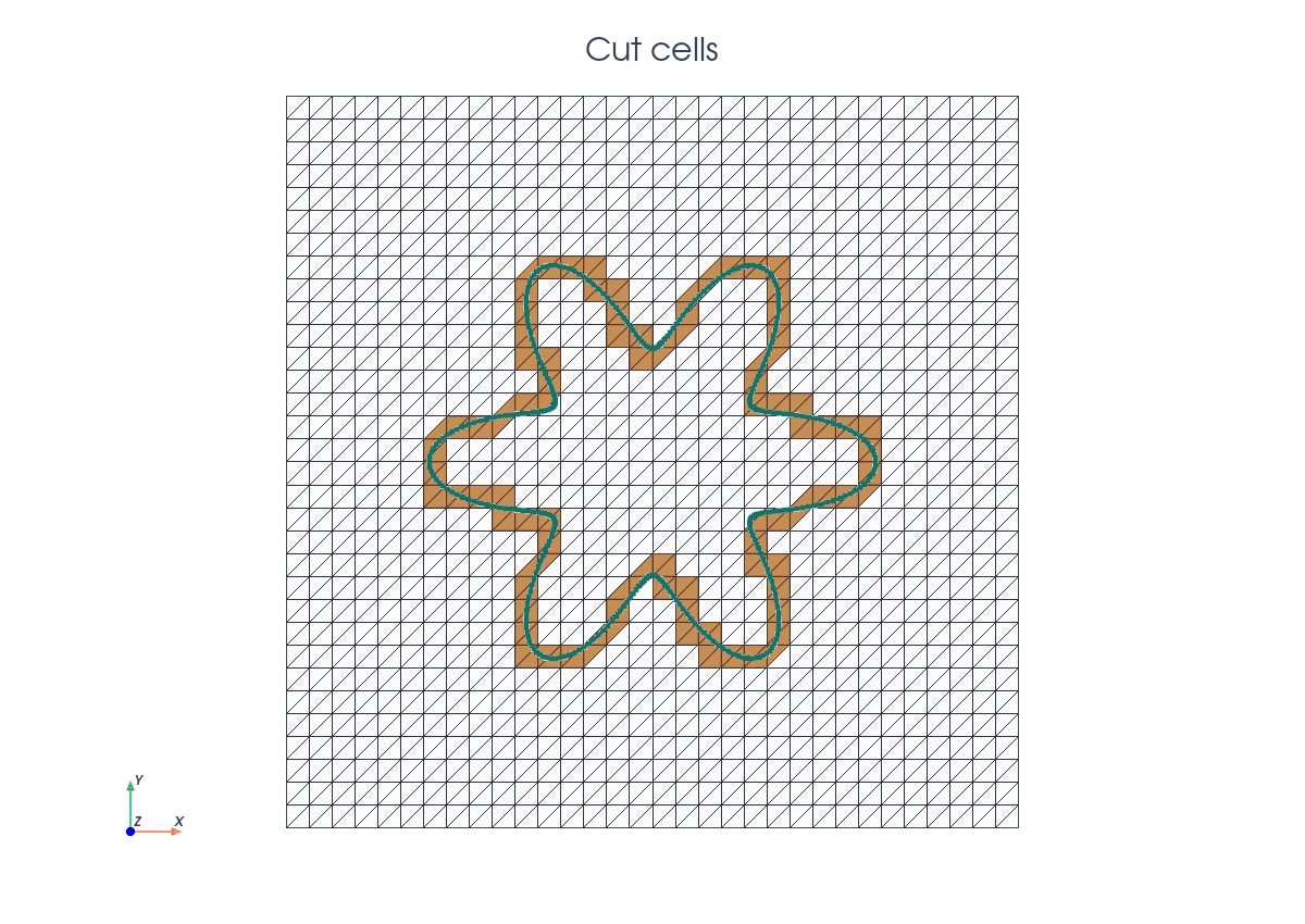
order = 4
volume_rules = cutfemx.runtime_quadrature(cut_data, "phi<0", order)
interface_rules = cutfemx.runtime_quadrature(cut_data, "phi=0", order)

Blue points indicate cut-volume quadrature; magenta points indicate embedded-boundary quadrature.

The standard cells and runtime rules are combined in UFL measures:

dx_omega = ufl.Measure(
    "dx", domain=msh, subdomain_id=0, subdomain_data=[inside_cells, volume_rules]
)
dx_gamma = ufl.Measure("dx", domain=msh, subdomain_id=1, subdomain_data=interface_rules)

Each integration measure needs a different subdomain_id.

Finite Element Space

The unknown is still a standard continuous Lagrange function on the background mesh. The restriction to \(\Omega\) is encoded by the measures and by degree-of-freedom deactivation after assembly.

V = fem.functionspace(msh, ("Lagrange", 1))
u = ufl.TrialFunction(V)
v = ufl.TestFunction(V)
x = ufl.SpatialCoordinate(msh)

u_exact = ufl.sin(np.pi * x[0]) * ufl.sin(np.pi * x[1])
f = 2.0 * np.pi**2 * u_exact

Nitsche Boundary Terms

The embedded boundary does not coincide with mesh facets. Therefore, we enforce Dirichlet conditions weakly using Nitsche’s method. For Nitsche’s method, we need the outside normal to the interface, which can be computed in CutFEMx from the level-set function with cutfemx.normal(phi). The weak formulation we want to implement is

\[ a(u, v) = \int_{\Omega} \nabla u \cdot \nabla v \, dx + \int_{\Gamma} \left( - (\nabla u \cdot n_{\Gamma}) v - (\nabla v \cdot n_{\Gamma}) u + \frac{\gamma}{h} u v \right) \, ds \]

\[ L(v) = \int_{\Omega} f v \, dx + \int_{\Gamma} \left( - (\nabla v \cdot n_{\Gamma}) u_{\mathrm{exact}} + \frac{\gamma}{h} u_{\mathrm{exact}} v \right) \, ds \]

n_gamma = cutfemx.normal(phi)
h = ufl.CellDiameter(msh)
gamma = 40.0

a = ufl.inner(ufl.grad(u), ufl.grad(v)) * dx_omega
a += (
    -ufl.dot(ufl.grad(u), n_gamma) * v
    - ufl.dot(ufl.grad(v), n_gamma) * u
    + gamma / h * u * v
) * dx_gamma

L = f * v * dx_omega
L += (-ufl.dot(ufl.grad(v), n_gamma) * u_exact + gamma / h * u_exact * v) * dx_gamma

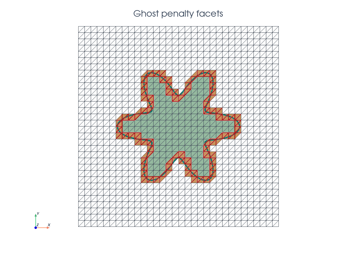
Ghost Penalty Facets

Small cuts can make the unstabilized stiffness matrix ill-conditioned. Here, we use ghost penalty stabilization, which adds gradient jump penalties to intersected edges and edges that connect intersected elements to the interior.

Red facets mark the ghost-penalty band coupling cut cells to neighboring active cells.

The ghost penalty terms are

\[ a(u, v) \mathrel{+}= \int_{\mathcal{F}_{\mathrm{ghost}}} \gamma_g h_{\mathrm{avg}} [\![ \nabla u \cdot n_F ]\!] [\![ \nabla v \cdot n_F ]\!] \, dS \]

which are implemented as

ghost_facets = cutfemx.ghost_penalty_facets(cut_data, "phi<0")
dS_ghost = ufl.Measure("dS", domain=msh, subdomain_id=2, subdomain_data=ghost_facets)

n_facet = ufl.FacetNormal(msh)
h_avg = ufl.avg(h)
gamma_g = 0.1

a += gamma_g * h_avg * ufl.inner( ufl.jump(ufl.grad(u), n_facet), ufl.jump(ufl.grad(v), n_facet),)* dS_ghost

Assembly And Solve

The UFL forms are compiled as CutFEMx runtime forms. After assembly, inactive background rows are replaced by identity rows so the serial sparse system has a well-defined value on every background degree of freedom.

a_form = cutfemx.fem.form(a)
L_form = cutfemx.fem.form(L)

A = cutfemx.fem.assemble_matrix(a_form)
A.scatter_reverse()
b = cutfemx.fem.assemble_vector(L_form)
b.scatter_reverse(la.InsertMode.add)
cutfemx.fem.deactivate_outside(A, b, cutfemx.fem.active_domain(a_form))

We solve the serial MatrixCSR system with SciPy:

from scipy.sparse.linalg import spsolve

uh = fem.Function(V, name="u_h")
uh.x.array[:] = spsolve(A.to_scipy().tocsr(), b.array)
uh.x.scatter_forward()

Then we compute the exact background function and the cut-domain error with the same dx_omega measure used for the solve:

u_exact_bg = fem.Function(V, name="u_exact")
u_exact_bg.interpolate(lambda x: np.sin(np.pi * x[0]) * np.sin(np.pi * x[1]))
u_exact_bg.x.scatter_forward()

error_bg = fem.Function(V, name="u_error")
error_bg.x.array[:] = uh.x.array - u_exact_bg.x.array
error_bg.x.scatter_forward()

error_form = cutfemx.fem.form((uh - u_exact) ** 2 * dx_omega)
error_sq = comm.allreduce(cutfemx.fem.assemble_scalar(error_form), op=MPI.SUM)

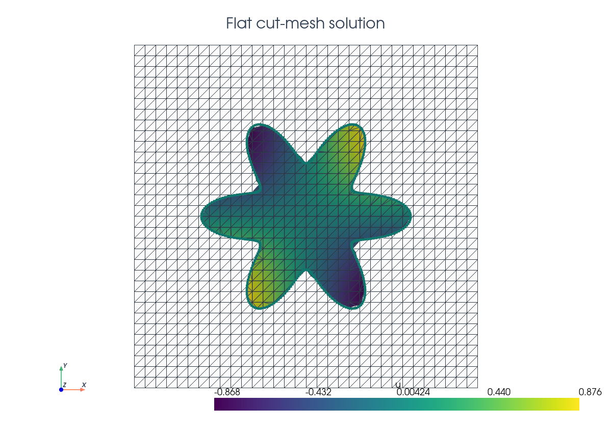
Solution Output

The solution is written both on the background mesh and on a visualization cut mesh. The cut mesh is not used for assembly; it is only a convenient output mesh for inspecting the physical domain.

Solution to Poisson problem on the flower-shaped cut mesh.

cut_mesh = cutfemx.create_cut_mesh(cut_data, "phi<0", mode="full")
uh_cut = cutfemx.fem.cut_function(uh, cut_mesh)

The script writes:

• poisson_xdmf/poisson_background.xdmf

• poisson_xdmf/poisson_cut_domain.xdmf

Related Literature

• E. Burman, S. Claus, P. Hansbo, M. G. Larson, and A. Massing, “CutFEM: Discretizing Geometry and Partial Differential Equations”, International Journal for Numerical Methods in Engineering 104(7), 472-501, 2015. This is the main CutFEM reference for the unfitted Nitsche formulation and ghost stabilization used in this example.

• E. Burman, “Ghost Penalty”, Comptes Rendus Mathematique 348(21-22), 1217-1220, 2010. This is the original short reference for the ghost-penalty stabilization used to keep cut-cell systems well conditioned.

• A. Hansbo and P. Hansbo, “An unfitted finite element method, based on Nitsche’s method, for elliptic interface problems”, Computer Methods in Applied Mechanics and Engineering 191(47-48), 5537-5552, 2002. This is a classical unfitted Nitsche reference behind the weak boundary and interface treatment used in CutFEM formulations.

Run The Demo

python python/demo/demo_poisson.py

Full Source

The complete source remains available in the repository: python/demo/demo_poisson.py.