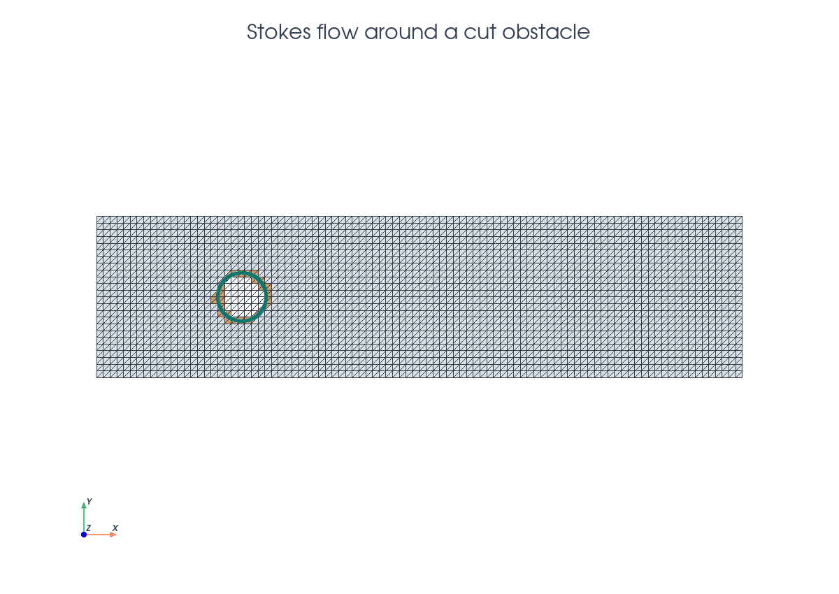
Stokes Flow

This tutorial follows python/demo/demo_stokes.py. It solves a steady channel Stokes problem with an unfitted circular obstacle. The inflow, walls, and outflow are fitted boundary facets of the rectangular mesh, while the obstacle boundary is represented by a level set and imposed weakly. The Nitsche fictitious-domain Stokes terms and the velocity/pressure stabilization are tied to the references listed in the related literature below.

Mesh for the Stokes flow around an obstacle. Orange cells are cut by the embedded circle.

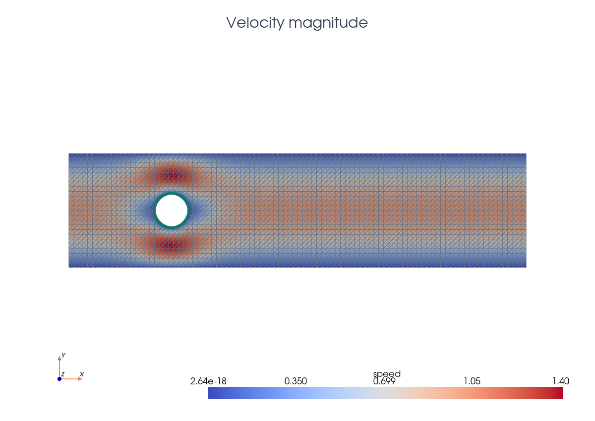
Model Problem

The fluid domain is

\[ \Omega=\{(x,y)\in[-3,5]\times[-1,1]:\phi(x,y)>0\}, \qquad \phi(x,y)=\sqrt{(x+1.2)^2+y^2}-0.3 . \]

The demo solves the steady Stokes equations,

\[ -\nu\Delta u+\nabla p=0,\qquad \nabla\cdot u=0 \quad\text{in }\Omega . \]

The fitted channel boundaries carry standard flow boundary conditions:

\[ u=(1-y^2,0)\quad\text{on }x=-3,\qquad u=0\quad\text{on }y=\pm1,\qquad p=0\quad\text{on }x=5 . \]

The circular obstacle has \(u=0\) on \(\Gamma=\{\phi=0\}\), imposed by Nitsche terms. The outflow pressure condition fixes the pressure reference on the fitted outlet. The velocity outflow condition remains natural in the weak form, so no strong velocity constraint is applied at \(x=5\).

Implementation Order

The demo executes the solve in this order:

1. Define the positive-in-fluid cylinder level set, gradient-form traction, serial solve helper, and XDMF writer.

2. Build the triangular channel mesh and equal-order mixed P1/P1 space.

3. Interpolate the pressure-space level set and cut the fluid domain.

4. Locate fluid/cut cells, build fluid/interface rules, ghost facets, and the active pressure-stabilization skeleton.

5. Build dx_omega, dx_gamma, dS_ghost, and dS_pressure.

6. Assemble the Stokes volume terms, obstacle Nitsche terms, velocity ghost penalty, and pressure gradient-jump stabilization.

7. Build fitted inflow/wall velocity boundary conditions and the fitted outflow pressure condition, assemble with BCs, apply lifting, deactivate inactive dofs, and solve.

8. Split velocity/pressure, interpolate velocity for XDMF compatibility, print diagnostics, and write background plus cut-fluid XDMF files.

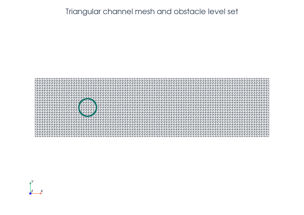
Triangular Channel Mesh

The mesh is created exactly as in the demo: a rectangle with 4*n cells in the streamwise direction and n cells across the channel, using triangular cells.

The obstacle cuts through the triangular channel mesh; no fitted circular boundary is inserted.

msh = mesh.create_rectangle(
    comm,
    ((-3.0, -1.0), (5.0, 1.0)),
    (4 * n, n),
    cell_type=mesh.CellType.triangle,
)

The velocity and pressure are both continuous P1 fields. The equal-order pair is stabilized by a pressure gradient-jump term on the active skeleton.

P1 = basix.ufl.element("Lagrange", msh.basix_cell(), 1)
P1_vec = basix.ufl.element(
    "Lagrange", msh.basix_cell(), 1, shape=(msh.geometry.dim,)
)
W = fem.functionspace(msh, basix.ufl.mixed_element([P1_vec, P1]))

Cut Fluid Domain

The positive phase is the fluid. Cut cells are handled separately because they need partial-volume and interface quadrature.

cylinder_center = (-1.2, 0.0)
cylinder_radius = 0.3

level_set = fem.Function(Q, name="phi")
level_set.interpolate(cylinder_level_set(cylinder_center, cylinder_radius))
level_set.x.scatter_forward()

cut_data = cutfemx.cut(level_set)
fluid_cells = cutfemx.locate_entities(cut_data, "phi>0")
cut_cells = cutfemx.locate_entities(cut_data, "phi=0")

The strict selector "phi>0" gives the ordinary fluid cells used with standard cell quadrature. The cut cells are not added as full cells in dx_omega; their fluid portions are integrated by the runtime quadrature rules below.

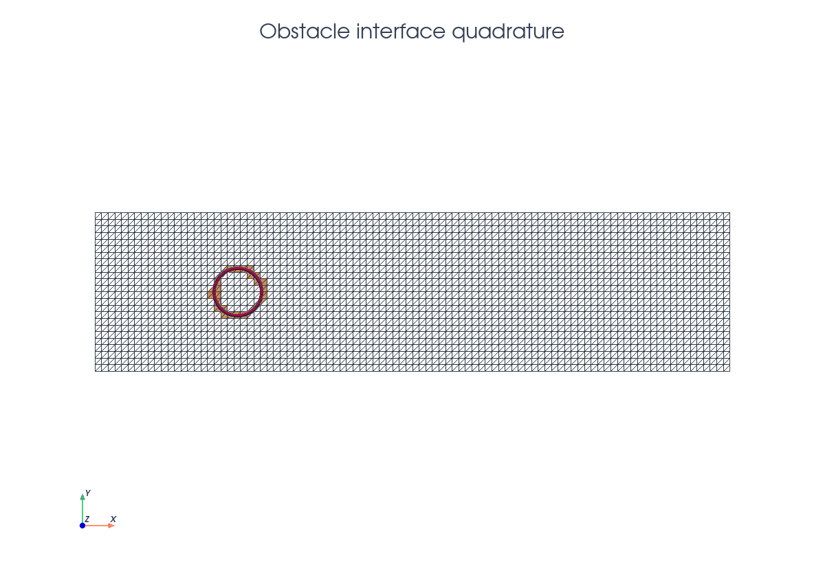
Interface Quadrature And Nitsche Terms

The obstacle boundary is not part of the mesh topology. CutFEMx supplies physical quadrature points on the embedded circle, and the normal is computed from the level set.

Magenta markers are the actual interface quadrature points used for obstacle Nitsche terms.

fluid_rules = cutfemx.runtime_quadrature(cut_data, "phi>0", order)
interface_rules = cutfemx.runtime_quadrature(cut_data, "phi=0", order)

dx_omega = ufl.Measure(
    "dx", domain=msh, subdomain_id=0, subdomain_data=[fluid_cells, fluid_rules]
)
dx_gamma = ufl.Measure("dx", domain=msh, subdomain_id=1, subdomain_data=interface_rules)
n_gamma = -cutfemx.normal(level_set)

Weak Formulation

Let \(V_h\) be the continuous P1 velocity space and \(Q_h\) the continuous P1 pressure space on the background mesh. Strong Dirichlet data are applied on the fitted inflow, wall, and outflow-pressure facets, so the corresponding test functions vanish there. No strong velocity condition is applied at the outflow.

The cut-domain volume contribution is the standard mixed Stokes form:

\[ a_\Omega((u,p),(v,q)) =\int_\Omega \nu\nabla u:\nabla v\,dx -\int_\Omega p\,\nabla\cdot v\,dx +\int_\Omega (\nabla\cdot u)q\,dx . \]

In code this is the first block of the bilinear form:

a = nu * ufl.inner(ufl.grad(u), ufl.grad(v)) * dx_omega
a += -p * ufl.div(v) * dx_omega
a += ufl.div(u) * q * dx_omega

The weak obstacle terms use the Stokes traction \(t(u,p)=(\nu\nabla u-pI)n_\Gamma\) and impose \(u=0\) on \(\Gamma=\{\phi=0\}\) by symmetric Nitsche terms:

\[ N_\Gamma((u,p),(v,q)) =-\int_\Gamma t(u,p)\cdot v\,d\Gamma -\int_\Gamma t(v,q)\cdot u\,d\Gamma +\int_\Gamma \frac{\gamma_u\nu}{h}u\cdot v\,d\Gamma . \]

def traction(u, p, nu, n):
    return nu * ufl.dot(ufl.grad(u), n) - p * n


a += -ufl.inner(traction(u, p, nu, n_gamma), v) * dx_gamma
a += -ufl.inner(traction(v, q, nu, n_gamma), u) * dx_gamma
a += gamma_u * nu / h * ufl.inner(u, v) * dx_gamma

The right-hand side is zero in this example,

\[ L(v,q)=\int_\Omega f\cdot v\,dx,\qquad f=(0,0), \]

because the flow is driven by the strong parabolic inflow condition.

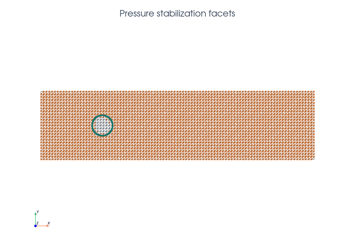
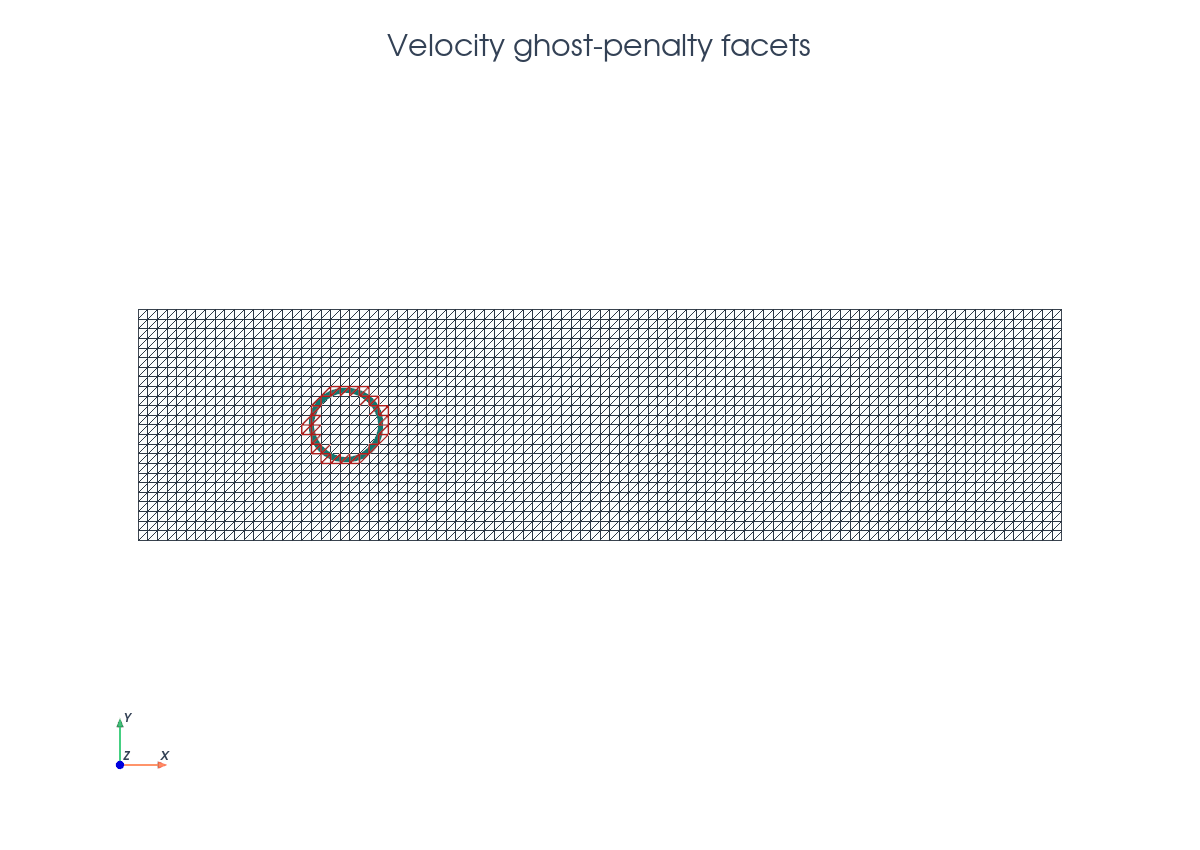
Stabilization Facets

The demo uses different facet sets for pressure and velocity stabilization. This separation matters: equal-order pressure stability is a global active skeleton requirement, while velocity stabilization is only needed to control small cut-cell extensions near the unfitted obstacle.

Orange facets are the active interior facets used by the pressure gradient-jump stabilization.

Red facets are the velocity ghost-penalty band around the cut obstacle cells.

ghost_facets = cutfemx.ghost_penalty_facets(cut_data, "phi>0")
active_cells = np.union1d(fluid_cells, cut_cells)
pressure_facets = cutfemx.interior_facets_for_cells(msh, active_cells)

dS_ghost = ufl.Measure("dS", domain=msh, subdomain_id=2, subdomain_data=ghost_facets)
dS_pressure = ufl.Measure("dS", domain=msh, subdomain_id=3, subdomain_data=pressure_facets)

Pressure Stabilization

The P1/P1 pair does not satisfy the inf-sup condition without additional stabilization. The demo therefore adds a pressure gradient-jump term on all active interior facets,

\[ \mathcal F_h^\Omega=\texttt{interior\_facets\_for\_cells(active\_cells)} . \]

The term is

\[ S_p(p,q)= \gamma_p\int_{\mathcal F_h^\Omega} h^3[\nabla p]n\cdot[\nabla q]n\,dS . \]

In the implementation this is the dS_pressure contribution

a += (
    gamma_p
    * ufl.avg(h) ** 3
    * ufl.inner(
        ufl.jump(ufl.grad(p), n_facet),
        ufl.jump(ufl.grad(q), n_facet),
    )
    * dS_pressure
)

Velocity Ghost Penalty

Velocity does not receive a gradient-jump term on the full active skeleton. Instead, it is stabilized only on the ghost-penalty band \(\mathcal F_g\) returned by ghost_penalty_facets(cut_data, "phi>0"). This band couples cut cells to neighboring fluid cells and controls conditioning when the circle leaves very small intersections.

\[ S_u(u,v)= \gamma_g\int_{\mathcal F_g} h[\nabla u]n\cdot[\nabla v]n\,dS . \]

The code deliberately uses dS_ghost, not dS_pressure, for this term:

if ghost_facets.size > 0:
    a += (
        gamma_g
        * ufl.avg(h)
        * ufl.inner(
            ufl.jump(ufl.grad(u), n_facet),
            ufl.jump(ufl.grad(v), n_facet),
        )
        * dS_ghost
    )

The full bilinear form is therefore

\[ A((u,p),(v,q)) =a_\Omega((u,p),(v,q)) +N_\Gamma((u,p),(v,q)) +S_p(p,q) +S_u(u,v). \]

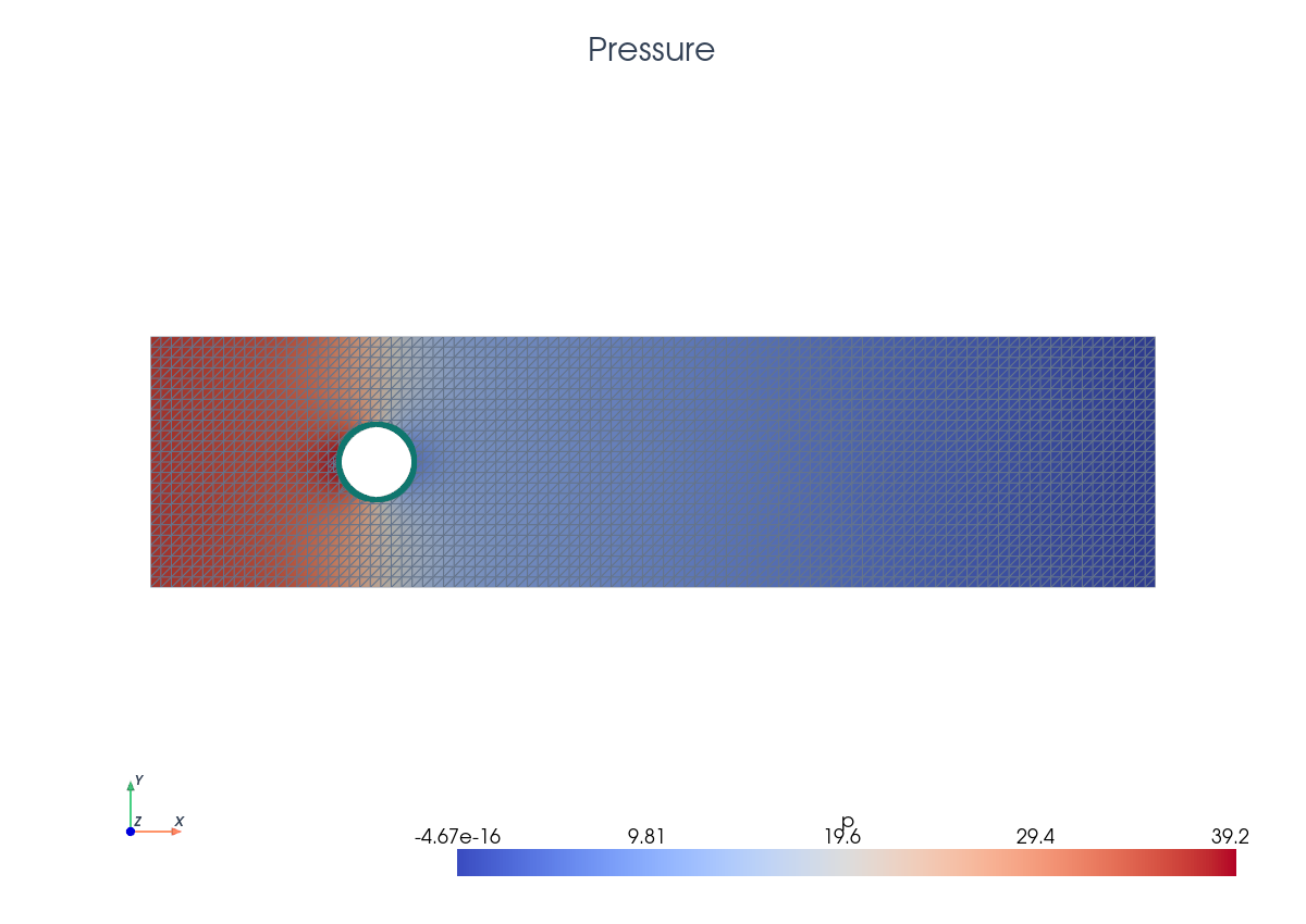
Boundary Conditions And Output

The strong boundary conditions are velocity conditions on the fitted inflow and channel walls, plus a pressure condition on the fitted outflow. The pressure condition fixes the pressure level and sets the outlet reference value to zero. After solving, CutFEMx writes both background and cut-fluid XDMF files.

inflow_u = fem.Function(V)
inflow_u.interpolate(lambda x: np.stack((1.0 - x[1] ** 2, np.zeros_like(x[0]))))
walls_u = fem.Function(V)
walls_u.x.array[:] = 0.0
outflow_p = fem.Function(Q)
outflow_p.x.array[:] = 0.0

inflow_facets = mesh.locate_entities_boundary(
    msh, facet_dim, lambda x: np.isclose(x[0], -3.0)
)
wall_facets = mesh.locate_entities_boundary(
    msh, facet_dim, lambda x: np.isclose(np.abs(x[1]), 1.0)
)
outflow_facets = mesh.locate_entities_boundary(
    msh, facet_dim, lambda x: np.isclose(x[0], 5.0)
)
inflow_dofs = fem.locate_dofs_topological((W.sub(0), V), facet_dim, inflow_facets)
wall_dofs = fem.locate_dofs_topological((W.sub(0), V), facet_dim, wall_facets)
outflow_pressure_dofs = fem.locate_dofs_topological(
    (W.sub(1), Q), facet_dim, outflow_facets
)

bcs = [
    fem.dirichletbc(inflow_u, inflow_dofs, W.sub(0)),
    fem.dirichletbc(walls_u, wall_dofs, W.sub(0)),
    fem.dirichletbc(outflow_p, outflow_pressure_dofs, W.sub(1)),
]

Deactivation

The Stokes unknown is a mixed background field, so the linear system contains velocity and pressure degrees of freedom on the whole rectangular mesh. The forms only integrate over the fluid phase \(\Omega=\{\phi>0\}\), which means degrees of freedom supported entirely inside the solid obstacle would otherwise produce empty matrix rows. These rows are not physical unknowns of the cut problem and must be deactivated before the sparse solve.

The active domain is computed from the assembled CutFEMx form. It includes the mixed dofs touched by the volume, interface, ghost-penalty, pressure stabilization, and fitted-boundary terms. After assembly, CutFEMx replaces inactive rows by identity rows and sets the corresponding right-hand-side entries consistently. This gives the serial sparse system a well-defined value for every background dof while leaving the active fluid equations unchanged.

The order is important when strong fitted boundary conditions are present: assemble with the velocity and pressure BCs, apply the usual lifting and boundary values, scatter the vector contributions, and only then deactivate inactive cut-domain dofs.

a_form = cutfemx.fem.form(a)
L_form = cutfemx.fem.form(L)

A = cutfemx.fem.assemble_matrix(a_form, bcs=bcs)
A.scatter_reverse()

b = cutfemx.fem.assemble_vector(L_form)
cutfemx.fem.apply_lifting(b.array, [a_form], [bcs])
b.scatter_reverse(la.InsertMode.add)
fem.set_bc(b.array, bcs)

active = cutfemx.fem.active_domain(a_form)
cutfemx.fem.deactivate_outside(A, b, active)

The fitted inflow, wall, and outflow-pressure dofs are still handled as ordinary DOLFINx Dirichlet conditions. Deactivation handles a different set of rows: mixed velocity-pressure dofs that are outside the active fluid problem because the obstacle cut removed their support.

Velocity magnitude on the cut-fluid mesh.

Pressure on the cut-fluid mesh with the fitted outflow pressure set to zero.

The script writes velocity and pressure fields in stokes_xdmf/.

Related Literature

• A. Massing, M. G. Larson, A. Logg, and M. E. Rognes, “A Stabilized Nitsche Fictitious Domain Method for the Stokes Problem”, Journal of Scientific Computing 61(3), 604-628, 2014. This is a core reference for unfitted Stokes discretizations with Nitsche boundary conditions, pressure stabilization, and ghost penalties.

• E. Burman, S. Claus, and A. Massing, “A Stabilized Cut Finite Element Method for the Three Field Stokes Problem”, SIAM Journal on Scientific Computing 37(4), A1705-A1726, 2015. This gives closely related CutFEM Stokes analysis with equal-order background fields, weak boundary imposition, and CIP/ghost-type stabilization.

Run The Demo

python python/demo/demo_stokes.py

Full Source

The complete source remains available in the repository: python/demo/demo_stokes.py.