Elasticity

This tutorial follows python/demo/demo_elasticity.py. The physical domain is a dogbone specimen cut from a tetrahedral background mesh. The left end is clamped, the right end is pulled in the \(x\) direction, and the solid domain is selected by the negative phase of a level set. The cut elasticity formulation is related to the linear-elasticity CutFEM analysis cited in the related literature below.

The final field is shown on the CutFEMx solid mesh extracted from the tetrahedral background mesh.

Model

The demo uses small-strain isotropic linear elasticity:

\[ \varepsilon(u)=\operatorname{sym}\nabla u,\qquad \sigma(u)=2\mu\varepsilon(u)+\lambda\operatorname{tr}(\varepsilon(u))I. \]

The weak form is

\[ \int_\Omega \sigma(u):\varepsilon(v)\,dx + a_\mathrm{ghost}(u,v) = \int_\Omega f\cdot v\,dx, \]

with zero body force in this demo.

Dogbone Level Set

The solid is defined by the negative phase of a P1 level-set function. For a point \(x=(x_0,x_1,x_2)\), the demo first computes a normalized axial coordinate

\[ t=\operatorname{clip}\left( \frac{|x_0|-\mathtt{gauge\_half\_length}} {\mathtt{half\_length}-\mathtt{gauge\_half\_length}}, 0,1 \right), \]

then applies a cubic smoothstep to make the shoulder transition smooth:

\[ s=t^2(3-2t),\qquad r(x_0)=\mathtt{waist\_radius} +(\mathtt{grip\_radius}-\mathtt{waist\_radius})s. \]

The level set is

\[ \phi(x)=\sqrt{x_1^2+x_2^2}-r(x_0), \]

so \(\phi<0\) selects the dogbone solid, \(\phi=0\) is the cut surface, and \(\phi>0\) is outside the specimen.

def dogbone_level_set(
    half_length: float,
    grip_radius: float,
    waist_radius: float,
    gauge_half_length: float,
):
    def phi(x: np.ndarray) -> np.ndarray:
        t = (np.abs(x[0]) - gauge_half_length) / (half_length - gauge_half_length)
        t = np.clip(t, 0.0, 1.0)
        shoulder = t * t * (3.0 - 2.0 * t)
        radius = waist_radius + (grip_radius - waist_radius) * shoulder
        return np.sqrt(x[1] ** 2 + x[2] ** 2) - radius

    return phi

Implementation Order

The demo runs in this order:

1. Define the dogbone level set.

2. Build the tetrahedral background mesh and interpolate the P1 level set.

3. Cut the solid, locate solid_cells, build solid_rules, and select ghost_facets.

4. Build dx_solid, dS_ghost, the vector Lagrange space, material constants, elasticity bilinear form, and zero body-force linear form.

5. Locate left/right fitted end facets and create the strong displacement boundary conditions.

6. Assemble with boundary conditions, apply lifting, deactivate inactive dofs, and solve the serial sparse system.

7. Interpolate a DG0 von Mises field, print diagnostics, and write both background and cut-solid XDMF outputs.

Tetrahedral Background And Cut Solid

The background mesh is a box of tetrahedra. The dogbone is represented by a smooth radius profile in the level-set function, not by a fitted surface mesh.

The visible solid is the generated CutFEMx cut mesh inside the tetrahedral background box.

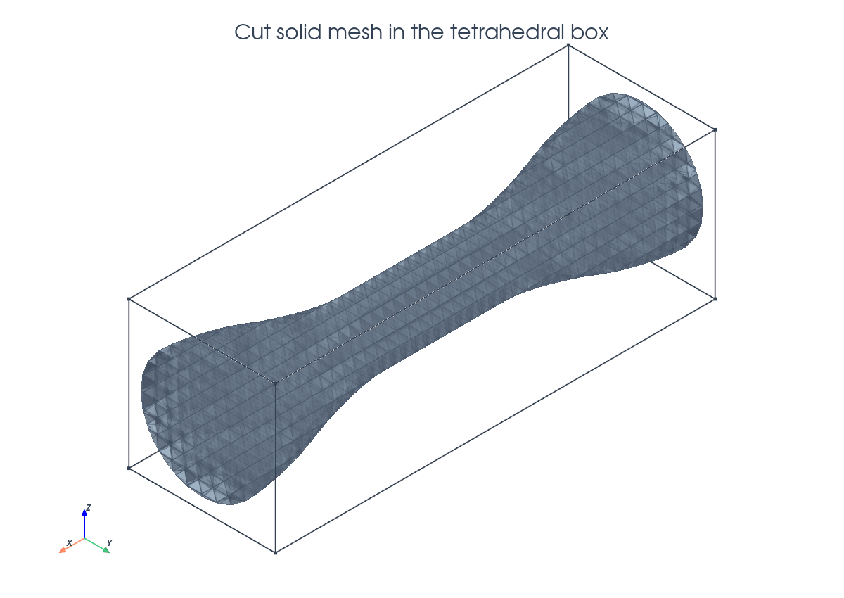
msh = mesh.create_box(
    comm,
    (
        np.array([-half_length, -box_radius, -box_radius]),
        np.array([half_length, box_radius, box_radius]),
    ),
    (4 * n, n, n),
    cell_type=mesh.CellType.tetrahedron,
)

phi = fem.Function(V_phi, name="phi")
phi.interpolate(dogbone_level_set(half_length, grip_radius, waist_radius, gauge_half_length))
phi.x.scatter_forward()

cut_data = cutfemx.cut(phi)
solid_cells = cutfemx.locate_entities(cut_data, "phi<0")

Cut-Volume Quadrature

The volume integral is evaluated on the part of each cut tetrahedron belonging to the solid. Interior solid cells and cut-cell runtime rules are combined in one measure.

Blue markers show a subsample of the physical cut-volume quadrature points.

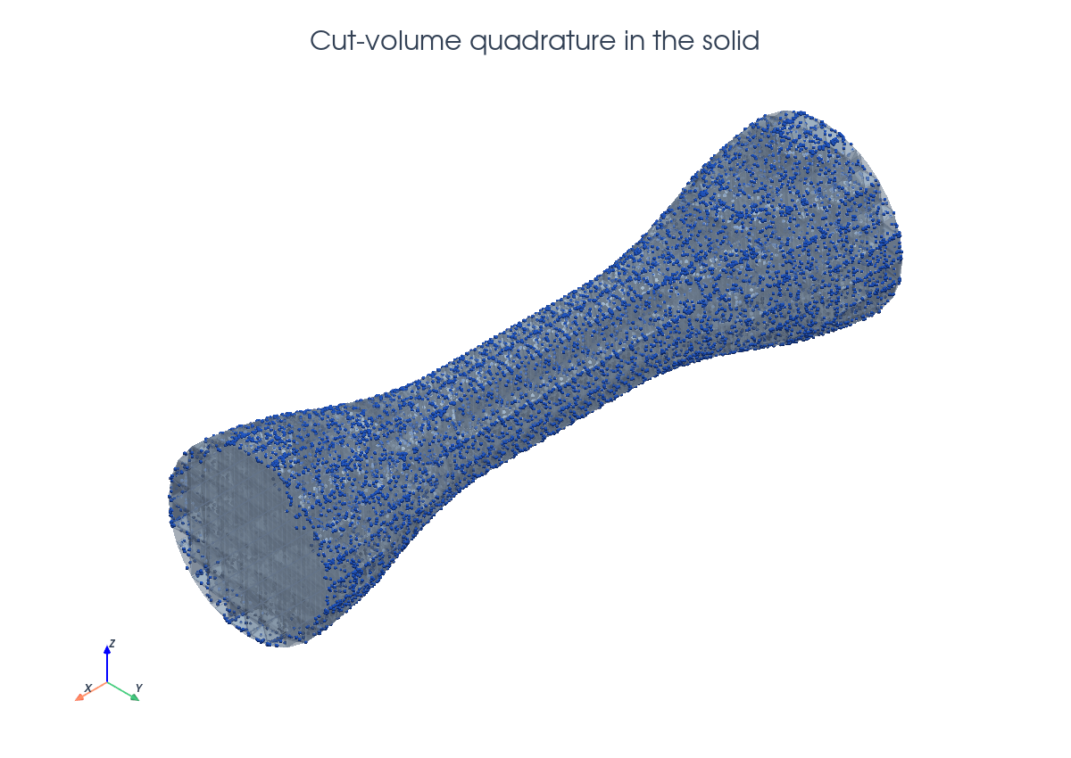
solid_rules = cutfemx.runtime_quadrature(cut_data, "phi<0", order)
dx_solid = ufl.Measure(
    "dx", domain=msh, subdomain_id=0, subdomain_data=[solid_cells, solid_rules]
)

Ghost Stabilization

The ghost penalty stabilizes displacement gradients across facets near the cut surface.

Red facets indicate the ghost-penalty facets selected around the cut solid.

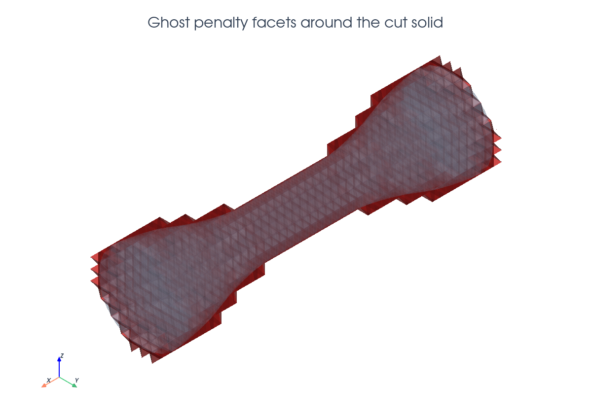
ghost_facets = cutfemx.ghost_penalty_facets(cut_data, "phi<0")
dS_ghost = ufl.Measure("dS", domain=msh, subdomain_id=1, subdomain_data=ghost_facets)

a = ufl.inner(sigma(u, mu, lmbda, gdim), epsilon(v)) * dx_solid
if ghost_facets.size > 0:
    n_facet = ufl.FacetNormal(msh)
    h_avg = ufl.avg(ufl.CellDiameter(msh))
    a += gamma_ghost * (2.0 * mu + lmbda) * h_avg * ufl.inner(
        ufl.jump(ufl.grad(u), n_facet),
        ufl.jump(ufl.grad(v), n_facet),
    ) * dS_ghost

Boundary Conditions

The mechanical boundary conditions are fitted on the box ends: all components are fixed on the left, and the \(x\) component is prescribed on the right.

left_facets = mesh.locate_entities_boundary(
    msh, facet_dim, lambda x: np.isclose(x[0], -half_length)
)
right_facets = mesh.locate_entities_boundary(
    msh, facet_dim, lambda x: np.isclose(x[0], half_length)
)

u_left = fem.Function(V)
left_dofs = fem.locate_dofs_topological(V, facet_dim, left_facets)
bcs = [fem.dirichletbc(u_left, left_dofs)]

Vx, _ = V.sub(0).collapse()
u_right_x = fem.Function(Vx)
u_right_x.interpolate(lambda x: pull * np.ones_like(x[0]))
right_x_dofs = fem.locate_dofs_topological((V.sub(0), Vx), facet_dim, right_facets)
bcs.append(fem.dirichletbc(u_right_x, right_x_dofs, V.sub(0)))

Assembly And Solve

The solver helper follows the actual CutFEMx MatrixCSR path. Boundary conditions are applied during matrix assembly, the right-hand side is lifted, inactive dofs are deactivated from the form active domain, and SciPy solves the serial sparse matrix.

a_form = cutfemx.fem.form(a)
L_form = cutfemx.fem.form(L)

A = cutfemx.fem.assemble_matrix(a_form, bcs=bcs)
A.scatter_reverse()
b = cutfemx.fem.assemble_vector(L_form)
cutfemx.fem.apply_lifting(b.array, [a_form], [bcs])
b.scatter_reverse(la.InsertMode.add)
fem.set_bc(b.array, bcs)

active = cutfemx.fem.active_domain(a_form)
cutfemx.fem.deactivate_outside(A, b, active)

uh = fem.Function(V, name="deformation")
uh.x.array[:] = spsolve(A.to_scipy().tocsr(), b.array)
uh.x.scatter_forward()

Stress Output

After solving, the demo derives a scalar von Mises stress field from the computed displacement. The stress tensor is first defined in UFL from the small-strain tensor,

def epsilon(u):
    return ufl.sym(ufl.grad(u))


def sigma(u, mu: float, lmbda: float, gdim: int):
    eps = epsilon(u)
    return 2.0 * mu * eps + lmbda * ufl.tr(eps) * ufl.Identity(gdim)

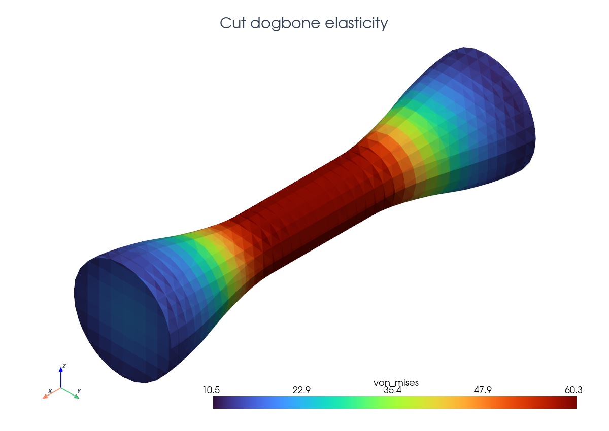
For this 3D example, the von Mises stress is the scalar UFL expression

\[ \sigma_\mathrm{vm} = \sqrt{ \frac{1}{2} \left[ (\sigma_{xx}-\sigma_{yy})^2 +(\sigma_{yy}-\sigma_{zz})^2 +(\sigma_{zz}-\sigma_{xx})^2 \right] +3\left(\sigma_{xy}^2+\sigma_{yz}^2+\sigma_{zx}^2\right) }. \]

The demo writes this definition directly in UFL:

def von_mises_3d(u, mu: float, lmbda: float):
    stress = sigma(u, mu, lmbda, 3)
    return ufl.sqrt(
        0.5
        * (
            (stress[0, 0] - stress[1, 1]) ** 2
            + (stress[1, 1] - stress[2, 2]) ** 2
            + (stress[2, 2] - stress[0, 0]) ** 2
        )
        + 3.0 * (stress[0, 1] ** 2 + stress[1, 2] ** 2 + stress[2, 0] ** 2)
    )

The output field is cellwise constant. The helper compute_von_mises_on_background_mesh creates a DG0 scalar space on the background mesh, converts the UFL expression to a dolfinx.fem.Expression at the DG0 interpolation points, and interpolates one value per background cell:

def compute_von_mises_on_background_mesh(
    u: fem.Function,
    mu: float,
    lmbda: float,
) -> fem.Function:
    msh = u.function_space.mesh
    Q = fem.functionspace(msh, ("Discontinuous Lagrange", 0))
    stress = fem.Function(Q, name="von_mises")

    interpolation_points = Q.element.interpolation_points
    if callable(interpolation_points):
        interpolation_points = interpolation_points()

    stress.interpolate(
        fem.Expression(von_mises_3d(u, mu, lmbda), interpolation_points)
    )
    return stress

This is an interpolation of the stress expression, not an additional variational projection. Since the displacement is P1, its gradient and the linear-elastic stress are cellwise constant on each background tetrahedron, so DG0 is the natural output space for this diagnostic.

The background DG0 field is then restricted to the physical cut-solid mesh with cutfemx.fem.cut_function before writing the cut-domain XDMF file:

von_mises = compute_von_mises_on_background_mesh(uh, mu, lmbda)

cut_mesh = cutfemx.create_cut_mesh(cut_data, "phi<0", mode="full")
stress_cut = cutfemx.fem.cut_function(von_mises, cut_mesh)
stress_cut.name = "von_mises"

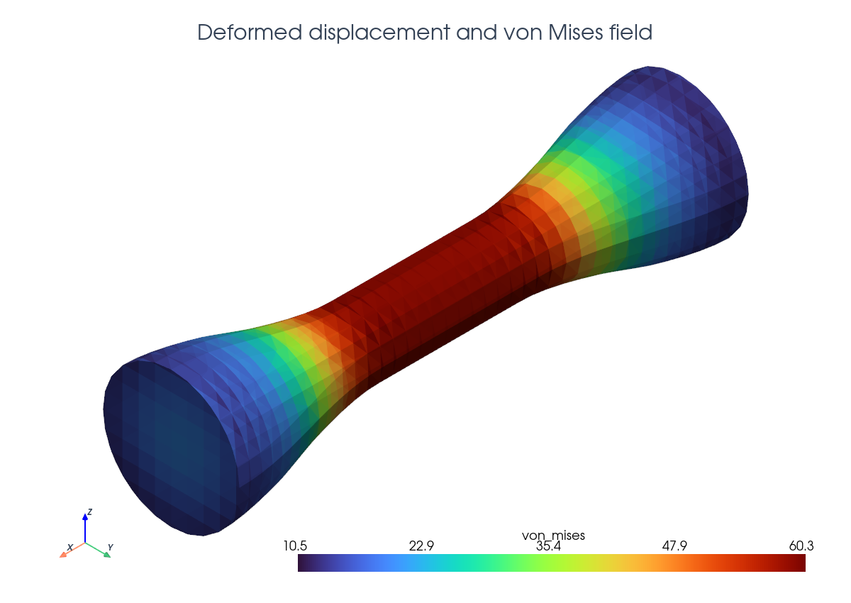
The tutorial view below shows the deformed cut mesh colored by that computed DG0 von Mises field.

The deformed CutFEMx solid mesh is color-mapped by the computed DG0 von Mises field.

The script writes background and cut-solid deformation and von Mises stress fields in elasticity_xdmf/.

Related Literature

• P. Hansbo, M. G. Larson, and K. Larsson, “Cut Finite Element Methods for Linear Elasticity Problems”, in Geometrically Unfitted Finite Element Methods and Applications, Lecture Notes in Computational Science and Engineering, 25-63, 2017. This chapter develops CutFEM formulations for linear elasticity on unfitted domains, including stabilization near the cut boundary and condition-number estimates.

• E. Burman, D. Elfverson, P. Hansbo, M. G. Larson, and K. Larsson, “Shape Optimization Using the Cut Finite Element Method”, Computer Methods in Applied Mechanics and Engineering 328, 242-261, 2018. This gives related elasticity examples where a level-set-defined elastic domain is evolved without remeshing.

Run The Demo

python python/demo/demo_elasticity.py

Full Source

The complete source remains available in the repository: python/demo/demo_elasticity.py.