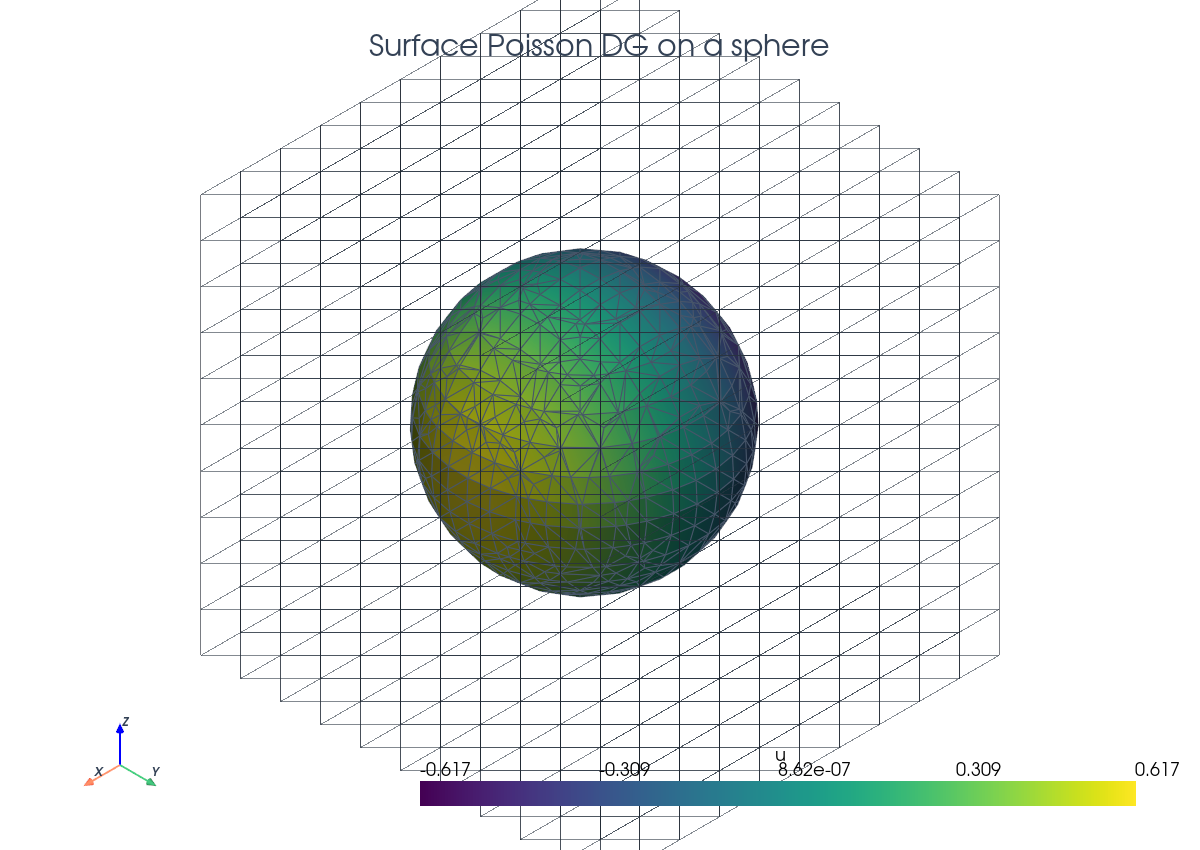
Surface Poisson DG

This tutorial follows python/demo/demo_surface_poisson_dg.py. The unknown is defined on an embedded surface rather than in one phase of a cut volume. The demo uses a hexahedral background mesh and builds the surface mesh from CutFEMx’s "phi=0" cut geometry. The surface CutFEM and cut DG ingredients are related to the references in the related literature below.

The CutFEMx surface mesh is extracted from the zero level set inside the hexahedral background mesh.

Model Problem

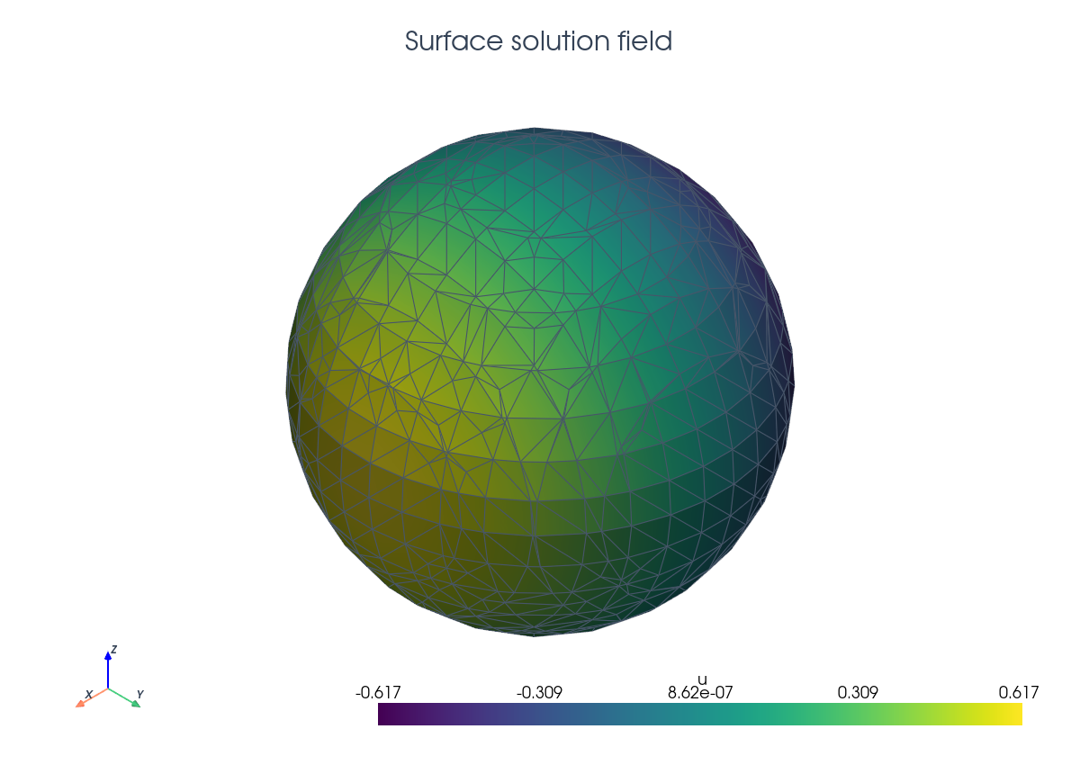
Let \(\Gamma=\{x:\phi(x)=0\}\) be a sphere of radius \(R=0.62\) centered at \(c=(0.05,-0.03,0.02)\). The demo solves

\[ -\Delta_\Gamma u + u = f \quad \text{on }\Gamma, \]

with manufactured solution \(u_\mathrm{ex}=x_0-c_0\). On the sphere this gives

\[ f=\left(1+\frac{2}{R^2}\right)(x_0-c_0). \]

Implementation Order

The demo executes the surface solve in this order:

1. Define the level set function.

2. Build the hexahedral background mesh and interpolate a quadratic level set.

3. Cut cells with "phi=0" and create Algoim surface quadrature.

4. Build the active surface skeleton by cutting interior facets adjacent to the cut cells; use those same surface skeleton facets as the ghost set.

5. Build dx_gamma, dS_gamma, and dS_ghost.

6. Build the DG space, tangential gradients, conormal jumps, SIPG terms, and ghost stabilization.

7. Assemble, deactivate inactive dofs, solve, compute exact/error fields and the surface measure, then write background, XDMF preview, and DG VTK output.

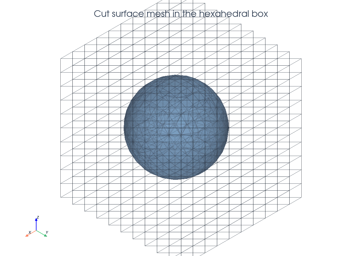
Background Mesh And Cut Surface

The level set is interpolated into a quadratic Lagrange space on the background hexahedral mesh. Cells intersected by the zero level set are found with the "phi=0" predicate.

The visible surface is the generated cut mesh, not an analytic sphere. The cut mesh is used only for visualisation. Quadrature rules are generated on the quadratic level set surface.

msh = mesh.create_box(
    comm,
    (np.array([-1.0, -1.0, -1.0]), np.array([1.0, 1.0, 1.0])),
    (n, n, n),
    cell_type=mesh.CellType.hexahedron,
)

V_phi = fem.functionspace(msh, ("Lagrange", 2))
phi = fem.Function(V_phi, name="phi")
phi.interpolate(lambda x: squared_distance(x, center) - radius**2)
phi.x.scatter_forward()

cell_cut = cutfemx.cut(phi)
cut_cells = cutfemx.locate_entities(cell_cut, "phi=0")

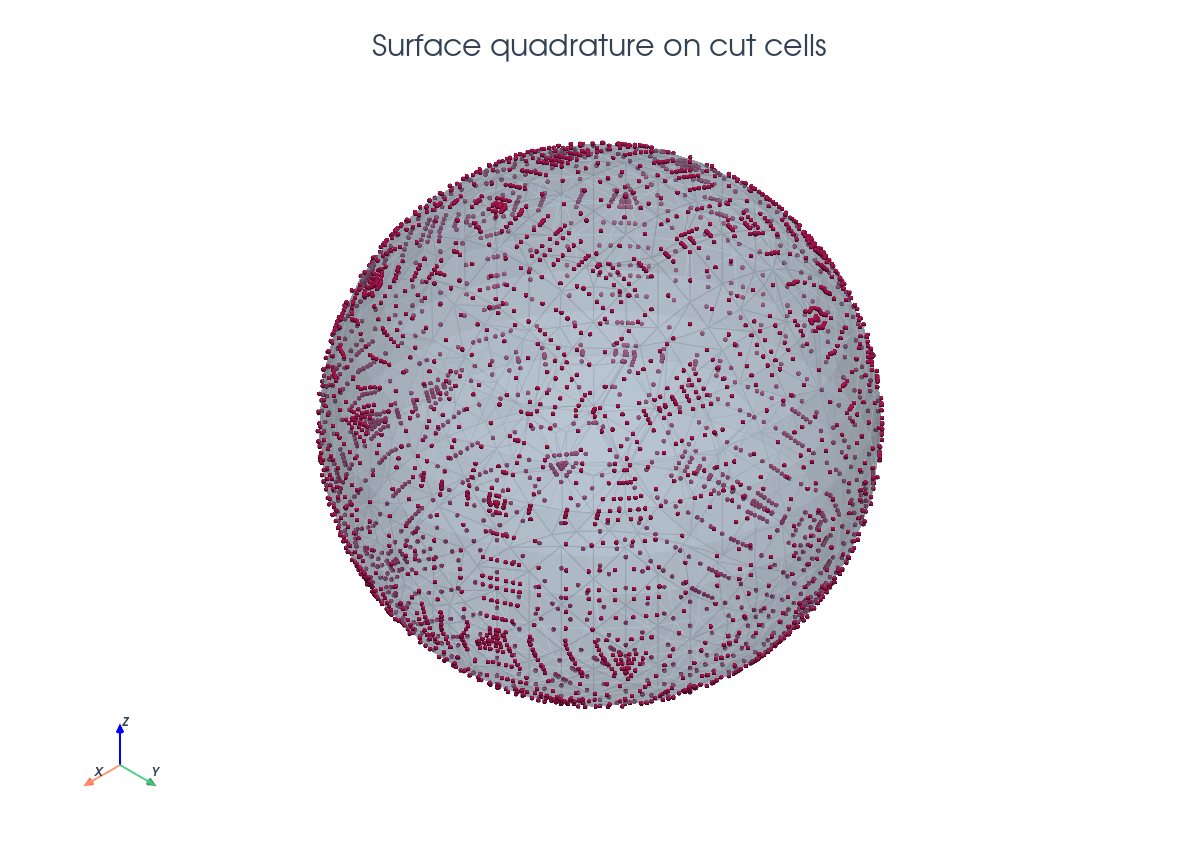
Surface Quadrature

CutFEMx generates quadrature points directly on \(\Gamma\cap K\) for each cut background cell. The demo uses the algoim backend for the surface rules.

Magenta points are the physical surface quadrature points returned by `runtime_quadrature`.

gamma_rules = cutfemx.runtime_quadrature(
    cell_cut, "phi=0", quadrature_order, backend="algoim"
)
dx_gamma = ufl.Measure("dx", domain=msh, subdomain_data=gamma_rules)

Tangential Differential Operators

The surface gradient is obtained by projecting the background gradient into the tangent plane:

\[ P=I-n_\Gamma\otimes n_\Gamma,\qquad \nabla_\Gamma u=P\nabla u . \]

n_gamma = cutfemx.normal(phi)
I = ufl.Identity(msh.geometry.dim)
P = I - ufl.outer(n_gamma, n_gamma)
grad_G_u = ufl.dot(P, ufl.grad(u))
grad_G_v = ufl.dot(P, ufl.grad(v))

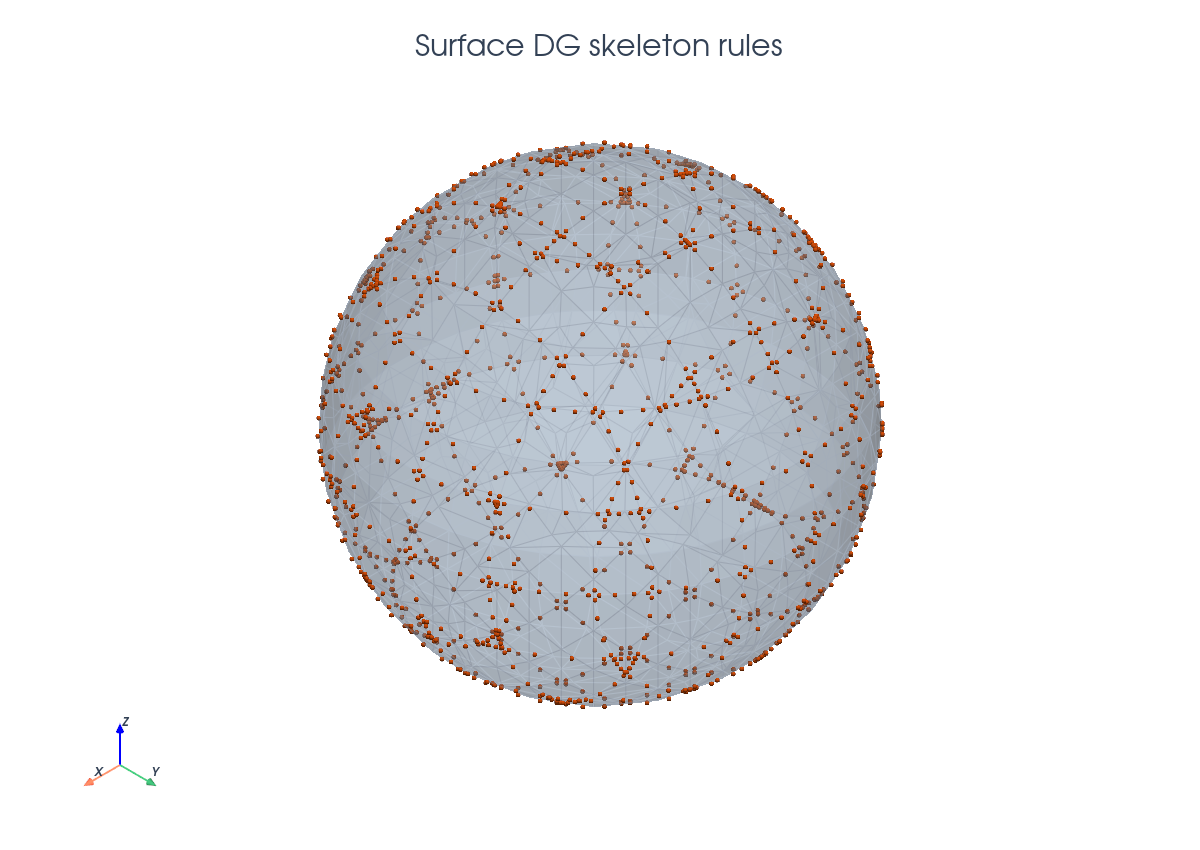
DG Skeleton On The Surface

The DG skeleton is formed from interior facets adjacent to cut cells. Those facets are cut again by the level set, this time as lower-dimensional entities.

Orange points show the physical quadrature locations for the cut surface skeleton rules.

skeleton_facets = cutfemx.interior_facets_for_cells(msh, cut_cells)
facet_cut = cutfemx.cut(phi, skeleton_facets, facet_dim)
skeleton_rules = cutfemx.runtime_quadrature(
    facet_cut, "phi=0", quadrature_order, backend="algoim"
)
ghost_facets = cutfemx.locate_entities(facet_cut, "phi=0")

dS_gamma = ufl.Measure("dS", domain=msh, subdomain_data=skeleton_rules)
dS_ghost = ufl.Measure("dS", domain=msh, subdomain_id=2, subdomain_data=ghost_facets)

The SIPG terms use conormals from CutFEMx:

mu = cutfemx.conormal(n_gamma)
jump_u_mu = ufl.jump(u, mu)
jump_v_mu = ufl.jump(v, mu)

Assembly And Output

The bilinear form combines the surface reaction-diffusion operator, skeleton consistency terms, SIPG penalty, and optional ghost stabilization:

\[ a(u,v)=\int_\Gamma (\nabla_\Gamma u\cdot\nabla_\Gamma v+uv)\,d\Gamma +a_\mathrm{SIPG}(u,v)+a_\mathrm{ghost}(u,v). \]

The forms are compiled as CutFEMx runtime forms, assembled into a serial sparse MatrixCSR system, and then deactivated outside the active surface problem before the SciPy solve. The computed surface field uh still lives on the background DG space; the cut-surface output step restricts it to the visualization mesh later.

a_form = cutfemx.fem.form(a)
L_form = cutfemx.fem.form(L)

A = cutfemx.fem.assemble_matrix(a_form)
A.scatter_reverse()
b = cutfemx.fem.assemble_vector(L_form)
b.scatter_reverse(la.InsertMode.add)

cutfemx.fem.deactivate_outside(A, b, cutfemx.fem.active_domain(a_form))

from scipy.sparse.linalg import spsolve

uh = fem.Function(V, name="u_h")
uh.x.array[:] = spsolve(A.to_scipy().tocsr(), b.array)
uh.x.scatter_forward()

The solution is color-mapped on the CutFEMx surface mesh.

The script writes:

• surface_poisson_dg_xdmf/surface_poisson_dg_background.xdmf

• surface_poisson_dg_xdmf/surface_poisson_dg_gamma.xdmf

• surface_poisson_dg_xdmf/surface_poisson_dg_gamma_dg.pvd

Related Literature

• E. Burman, P. Hansbo, M. G. Larson, and A. Massing, “A Cut Discontinuous Galerkin Method for the Laplace-Beltrami Operator”, IMA Journal of Numerical Analysis 37(1), 138-169, 2017. This is the direct reference for cut DG discretizations of surface Laplace-Beltrami type operators.

• E. Burman, P. Hansbo, M. G. Larson, and A. Massing, “Cut Finite Element Methods for Partial Differential Equations on Embedded Manifolds of Arbitrary Codimensions”, ESAIM: Mathematical Modelling and Numerical Analysis 52(6), 2247-2282, 2018. This gives the broader CutFEM framework for PDEs posed on embedded manifolds.

Run The Demo

python python/demo/demo_surface_poisson_dg.py

Full Source

The complete source remains available in the repository: python/demo/demo_surface_poisson_dg.py.