Compression

This tutorial follows python/demo/demo_compression.py. A rule of order 8 on a cut cell has hundreds or thousands of points, and most of them repeat information. If only some moments matter, for example those of a mass matrix, a small subset of the points with new weights gives the same integrals.

The volume rule of one cut reference cell at order 6, before and after compression onto degree 4. The colour is the weight, from small (dark) to large (light). The compressed points are a subset of the original ones, so they stay inside the part.

Usage

rules = result[phi < 0].quadrature(order=8, mode="cut_only")
small, stats = cutcells.compress_rules(rules, degree=4, space="total")
print(stats.points_before, stats.points_after, stats.max_residual)

degree and space give the polynomials whose moments are kept: "total" for total degree, usual on simplices, and "tensor" for the degree in each coordinate, usual on quadrilaterals and hexahedra. A rule then needs at most as many points as there are polynomials, whichever generator produced it. The result has the same fields as rules.

How Far the Points Fall

On the ball with a P2 level set and 9 grid points per side, order 8, compressed onto degree 4:

         shape     part   space  moments  before   after  ms/rule  residual
      triangle   volume   total       15      56      15     0.17   6.1e-16
      triangle  surface   total       15       7       7     0.00   0.0e+00
 quadrilateral   volume  tensor       25      50      25     0.13   5.0e-16
 quadrilateral  surface  tensor       25       9       9     0.00   0.0e+00
   tetrahedron   volume   total       35    1276      35     2.24   1.1e-15
   tetrahedron  surface   total       35      89      25     0.28   7.5e-13
    hexahedron   volume  tensor      125    1066     125    70.26   2.2e-14
    hexahedron  surface  tensor      125     102      77     1.39   3.4e-11
         prism   volume  tensor      125    1246     125    78.43   3.4e-13
         prism  surface  tensor      125     101      71     1.54   4.7e-11
       pyramid   volume  tensor      125    3034     125    97.24   3.0e-13
       pyramid  surface  tensor      125     296      86     4.73   5.4e-11

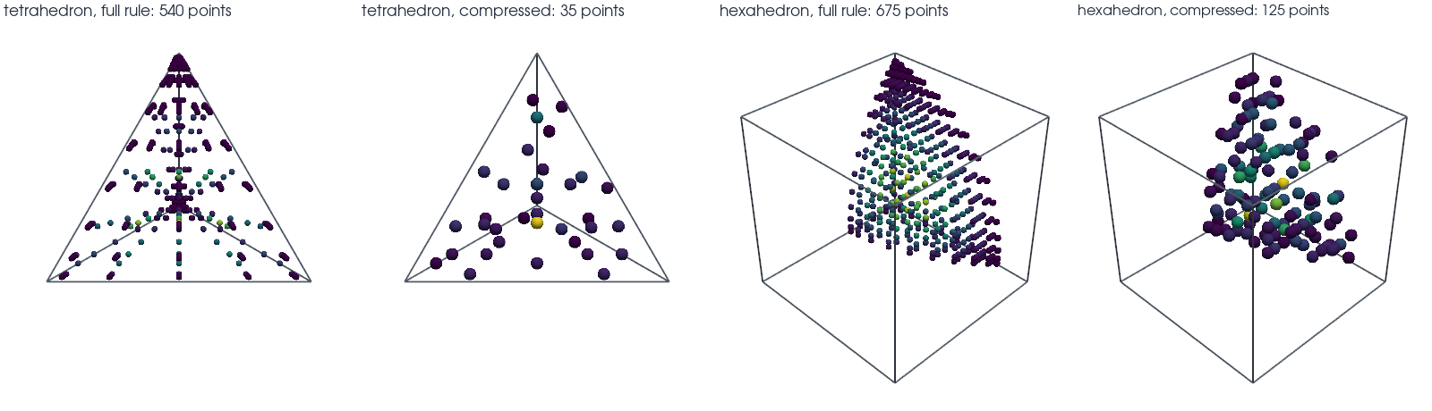
A tetrahedron goes from 1276 points to 35, a factor of 36. A hexahedron goes to 125, because the tensor space has more moments, and that is more costly to compute too. 2D rules gain less, since they start small. Only rules with more points than moments are compressed; the others are copied as they are, as on the 2D surfaces here. How many that leaves depends on the part: at order 4 onto degree 4, every volume rule of a cut tetrahedron is compressed, about 60 % of those of hexahedra and prisms, and 0 to 18 % of the surface rules in 3D. On a surface the moments are not independent, so the points stop below the moment count.

Mass Matrices

The mass matrix of degree \(k\) needs the moments of degree \(2k\). In each cut cell the demo assembles the matrix in a monomial basis with the full rule (order 8) and with the compressed one, in NumPy:

         shape  k          points  difference   compress  assemble, full  compressed  pays after
   tetrahedron  1      1276 -> 10     7.6e-15     0.30ms          0.36ms      0.06ms         1.0
   tetrahedron  2      1276 -> 35     7.4e-15     0.89ms          0.96ms      0.14ms         1.1
   tetrahedron  3      1276 -> 84     1.1e-12    10.42ms          2.18ms      0.34ms         5.7
    hexahedron  1      1066 -> 27     4.4e-15     0.47ms          0.71ms      0.11ms         0.8
    hexahedron  2     1066 -> 125     1.0e-14    29.27ms          3.51ms      0.69ms        10.4
    hexahedron  3     1066 -> 331     1.7e-11   103.59ms          6.74ms      2.47ms        24.2

difference is the largest change of an entry relative to the largest entry, over the cells. The matrices are unchanged to near round-off. pays after is how many assemblies with the compressed rule repay its cost. At low degree that is a single assembly. For Q3 on hexahedra it takes about 24. These times depend on the assembly: C++ assembly per point is faster, so compression pays later there.

What It Gives Up

Compression keeps only the chosen moments. An integrand beyond that degree is integrated less accurately than with the full rule, for example a mass matrix of degree 2 with a coefficient that is no polynomial:

         shape  degree  points    exp(x + y + z)   1 / (1 + 4 r^2)
   tetrahedron       4      35           4.6e-04           4.4e-03
   tetrahedron       6      84           1.6e-06           3.6e-04
   tetrahedron       8     162           2.8e-09           2.5e-05
    hexahedron       4     125           2.0e-03           1.4e-03
    hexahedron       6     331           4.4e-06           1.0e-04
    hexahedron       8     588           1.2e-08           3.4e-06

These are differences from the full rule, measured like the matrices above. With only the matrix’s own degree 4, two to three digits remain. The exponential gains a little under three digits for each two degrees, and the rational function about one.

Choosing the degree

Compress onto the degree of the whole integrand: twice the basis degree plus what you need for the coefficient, and check the difference on one cell. Compress once and reuse the rule when the geometry stays fixed over many assemblies, as in a time step or a Newton iteration. If the geometry moves every step, compression pays only at low degree.

Run the Demo

python python/demo/demo_compression.py
python python/demo/demo_compression.py --n 5 --order 6 --no-plot

Options: --n grid points per side, --order of the rules that are compressed, --no-plot to skip the PyVista window and --screenshot file.png to save the view.