Convergence

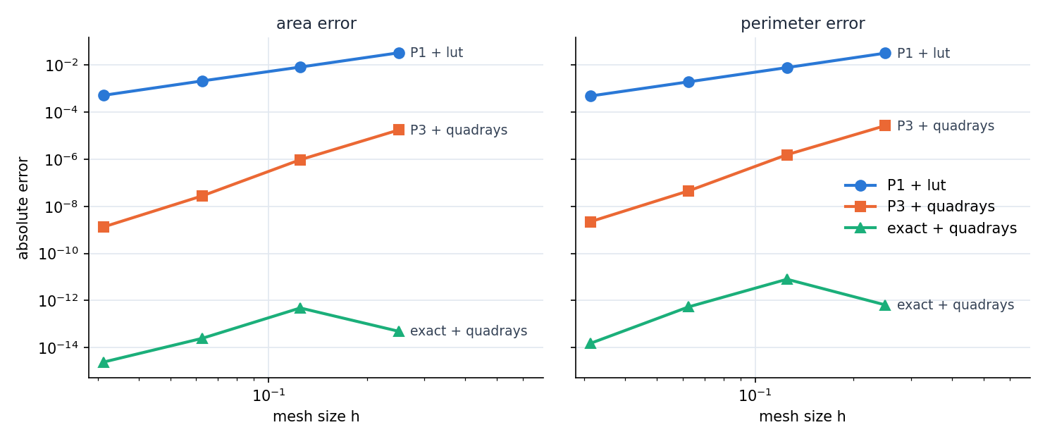
This tutorial follows python/demo/demo_convergence.py. It measures how the area and the perimeter of a disk converge under mesh refinement, for three ways of describing and integrating the disk.

Area and perimeter errors against the mesh size h, on triangular meshes of [-1, 1]^2.

Three Descriptions

The disk is the one of the previous chapter, \(\{|x-c|<R\}\) with \(R=0.6\), on triangular meshes of size \(h=2/(n-1)\).

P1 + lut

A P1 level set, integrated on the straight pieces of the lookup tables. The pieces are polygons inscribed in the circle; the error decays as \(h^2\).

P3 + quadrays

A P3 level set, integrated by quadrays on the curved pieces. quadrays integrates the region of the interpolant to the quadrature order, so the error is the interpolation error of the level set, \(h^{k+1}=h^4\).

exact + quadrays

The analytic circle cutcells.analytic_sphere, integrated by quadrays. The geometry is exact, only the quadrature error remains, and it is near round-off on every mesh.

Implementation

The three level sets differ only in how they are made and in the backend passed to cut:

def level_set(mesh, method):
    if method == "P1 + lut":
        return cutcells.create_level_set(mesh, circle, degree=1, name="phi"), "lut"
    if method == "P3 + quadrays":
        return cutcells.create_level_set(mesh, circle, degree=3, name="phi"), "quadrays"
    exact = cutcells.analytic_sphere([CENTER[0], CENTER[1], 0.0], RADIUS, name="phi")
    return exact, "quadrays"

and the rest of the study is the same for all of them:

for n in sizes:
    mesh = cutcells.rectangle_mesh(-1.0, -1.0, 1.0, 1.0, n, n, cell_type="triangle")
    for method in METHODS:
        phi, backend = level_set(mesh, method)
        result = cutcells.cut(mesh, phi, backend=backend)
        area = result[phi < 0].quadrature(order=order).weights.sum()
        perimeter = result[phi == 0].quadrature(order=order).weights.sum()

An analytic sphere in 2D is a disk; its centre takes three coordinates, of which the third is ignored.

Results

area error (rate)
        h                  P1 + lut             P3 + quadrays          exact + quadrays
   0.2500         3.271e-02                 1.731e-05                 1.178e-12        
   0.1250         7.739e-03 ( 2.03)         1.547e-06 ( 4.10)         7.999e-12 (-3.34)
   0.1250         8.127e-03 ( 2.01)         9.483e-07 ( 4.19)         4.834e-13 ( 1.28)
   0.0625         2.085e-03 ( 1.96)         2.738e-08 ( 5.11)         2.465e-14 ( 4.29)

perimeter error (rate)
        h                  P1 + lut             P3 + quadrays          exact + quadrays
   0.2500         3.170e-02                 2.650e-05                 7.923e-13        
   0.1250         7.739e-03 ( 2.03)         1.547e-06 ( 4.10)         7.998e-12 (-3.62)
   0.0312         5.136e-04 ( 2.02)         1.330e-09 ( 4.36)         2.442e-15 ( 3.33)
   0.0625         1.921e-03 ( 2.01)         4.509e-08 ( 5.10)         5.373e-13 ( 3.90)

The straight pieces converge with rate 2 and the interpolated level set with rate 4. With exact geometry the quadrature error is below \(10^{-11}\) on every mesh, and its rates say nothing: quadrays takes the points of the segments near the circle’s turning points in a variable anchored there (see Curved pieces in 3D below).

Reading the rates

The rate of the interpolated level set fluctuates around \(k+1\) on single steps: its error comes from the interpolation error along the curve, which partly cancels on coarse meshes. Over a longer range the rate settles: for P3, from \(n=17\) to \(n=513\) the errors are 9.5e-7, 2.7e-8, 1.3e-9, 1.9e-10, 1.3e-11 and 7.8e-13, rate 4.0 on average and 4.04 on the last step. Changing the quadrature order, the points per segment or the quadrays margin does not change these errors: they belong to the interpolant, not to the quadrature.

Curved pieces in 3D

quadrays bisects a box until the zero set’s normal has a margin along one axis; that sizes its leaves by the geometry, not by \(h\), and nested meshes bring the same leaves back. The margin bounds the slope of the height functions, not how close their turning points come: where a cell face cuts a sphere near its pole, the zero set on the face is a circle of any radius, whose turning point can lie just beyond a box, and so can the sphere’s silhouette seen along the height direction. At such a fold the height function has a square-root branch point, and the order’s Gauss-Legendre points converge slowly near it, on every mesh. So quadrays finds the folds near each curved box and takes the points of the segments that end within four lengths of one in \(s\) with \(x = x_f \mp s^2\) anchored at the fold \(x_f\), in which the integrand is smooth (QuadraysOptions.anchor_folds). Anchoring leaves about the same error on every mesh, so quadrays also checks each curved box against one more point per segment and bisects it while the two differ by more than the order’s own rate allows at the cell’s size, \((h\kappa/2)^{2q}\) for curvature \(\kappa\); pieces that converge as they should get no extra points, flat pieces are not checked. An anchored rule integrates the measure better than it does a polynomial, so on a box with anchored segments the check also compares a moment of what a mass matrix sees (QuadraysOptions.moment_tolerance). A box that fails first takes twice the points on those segments, which keeps polynomials of the order exact there, and is bisected only if that fails too.

For the sphere of radius 0.6 about \((0.1, -0.05, 0.03)\) in \([-1, 1]^3\) at order=6, the error of the area summed over the cells:

                       n = 5      n = 9     n = 17     n = 33     n = 65
hexahedra
  plain points         4.9e-06    6.2e-06    5.1e-06    4.0e-07    4.8e-09
  the check alone      4.9e-06    9.1e-07    1.3e-08    5.1e-11    3.4e-13
  anchored alone       2.1e-08    1.1e-08    1.1e-09    1.1e-10    1.9e-11
  twice the points     2.7e-12    1.4e-12    6.5e-12    2.1e-11    3.0e-13
  the default          5.5e-10    2.5e-11    6.2e-12    1.6e-11    3.1e-13
tetrahedra
  plain points         5.7e-06    5.2e-06    2.3e-06    1.5e-07    3.4e-08
  the check alone      5.2e-06    1.3e-06    1.8e-08    9.0e-11    2.5e-11
  anchored alone       9.6e-07    8.4e-09    7.2e-09    5.8e-09    1.9e-09
  twice the points     1.4e-11    7.1e-12    1.4e-11    1.4e-11    2.5e-11
  the default          3.7e-09    2.7e-10    1.3e-10    1.8e-11    2.5e-11

The total over the mesh hides most of this: cells that share a face near a pole err by opposite amounts. “Twice the points” is anchor_folds = 2 with the check on the measure alone, which keeps polynomials exact on every anchored segment. The default starts from one factor, and takes 0.55 to 1.2 times its points, mostly fewer on coarse meshes, where its error is up to some hundred times larger and still far below that of the check alone. It takes 0.8 to 2.6 times the points of plain points and 1.6 to 7.7 times their time. QuadraysOptions.anchor_folds = 0 gives plain points, tolerance sets a relative accuracy instead of the order’s rate (negative: no check), and points_per_segment still fixes the points for studies.

Run the Demo

python python/demo/demo_convergence.py
python python/demo/demo_convergence.py --sizes 17 33 65 129 257 --no-plot

Options: --sizes grid points per side of the meshes, --order of the quadrature, --no-plot to skip the matplotlib window and --screenshot file.png to save the plot.