Disk in a square#
This tutorial follows python/demo/demo_disk.py. It goes through the whole
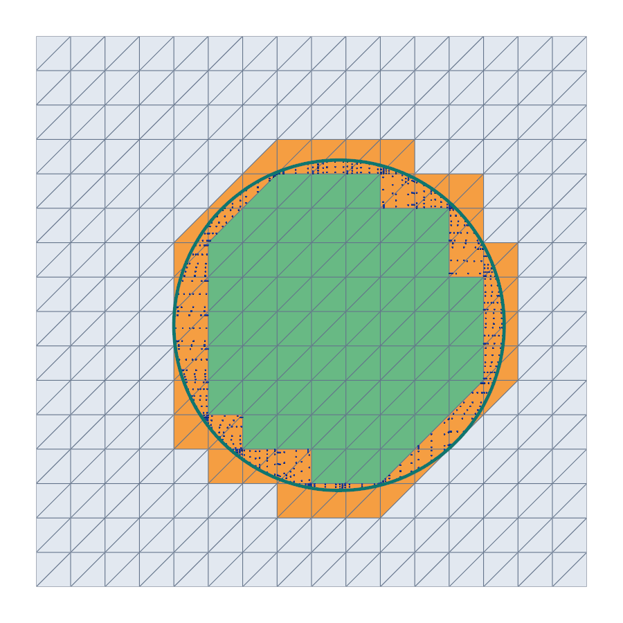
CutCells workflow in 2D: cut a triangular mesh by a circle, select the parts
on either side and on the circle, and integrate over them.
Geometry#
The background mesh covers the square \([-1,1]^2\). The circle of radius \(R\) about \(c\) is the zero set of the signed distance
which splits the square into three parts:
The demo checks three integrals against their exact values:
Implementation Order#
Build a structured triangular
MeshView.Interpolate \(\phi\) as a P2 level set named
phi.Call
cutcells.cutand selectphi < 0,phi == 0andphi > 0.Build quadrature rules for the disk and the circle and sum their weights.
Map the quadrature points to physical space and integrate \(|x-c|^2\).
Write the parts as VTU files and show them with PyVista.
Background Mesh#
A MeshView holds the background mesh as flat arrays: coordinates,
connectivity, offsets and cell types. rectangle_mesh builds one on a
rectangle with NumPy, splitting each grid square into two triangles; the
MeshView holds the NumPy arrays it built.
import numpy as np
import cutcells

mesh = cutcells.rectangle_mesh(-1.0, -1.0, 1.0, 1.0, n, n, cell_type="triangle")
n is the number of grid points per side; the demo’s default n = 25 gives
1152 triangles.
Level Set#
create_level_set interpolates a function on the mesh. The function receives
all interpolation points at once, as an array of shape (gdim, num_points),
and returns one value per point:
CENTER = (0.1, -0.05)
RADIUS = 0.6


def circle(X):
    return np.sqrt((X[0] - CENTER[0]) ** 2 + (X[1] - CENTER[1]) ** 2) - RADIUS


phi = cutcells.create_level_set(mesh, circle, degree=2, name="phi")
The name is the level set’s name in selection strings ("phi < 0") and in
the result.
Cut and Select#
cut classifies every cell by the level set: inside, cut, or outside. Indexing
the result with a condition built from the level set selects a part:
result = cutcells.cut(mesh, phi)

inside = result[phi < 0]
interface = result[phi == 0]
outside = result[phi > 0]
A part knows its dimension, 2 for the disk and 1 for the circle, and its
cells: inside.uncut_cells lie wholly inside, inside.cut_cells are the cut
cells of which it holds a piece. The colours of the figure are
result.domains[0], per cell 0 (inside), 1 (cut) or 2 (outside).
Quadrature#
part.quadrature(order) returns one quadrature rule per cell. With
mode="full" the disk’s rules cover its whole cells as well as its pieces of
the cut cells; the weights are physical, so they sum to the area:
inside_rules = inside.quadrature(order=4, mode="full")
interface_rules = interface.quadrature(order=4)

area = inside_rules.weights.sum()
perimeter = interface_rules.weights.sum()
By default the pieces are integrated with quadrays, which follows the
curved zero set of the P2 level set. order is the polynomial degree
integrated exactly on flat pieces.
Integrating a Function#
The points of a rule are given in the reference coordinates of its cell,
rules.parent_map gives the cell of each rule and rules.offset the points
of each rule. On a simplex mesh the affine map of each cell takes them to
physical space:
def physical_points(mesh, rules):
    tdim = rules.tdim
    reference = rules.points.reshape(-1, tdim)
    cells = np.repeat(rules.parent_map, np.diff(rules.offset))
    nodes = mesh.connectivity.reshape(-1, tdim + 1)[cells]
    x = mesh.coordinates[nodes]  # (num_points, tdim + 1, gdim)
    return x[:, 0] + np.einsum("pi,pig->pg", reference, x[:, 1:] - x[:, :1])


x = physical_points(mesh, inside_rules)
f = (x[:, 0] - CENTER[0]) ** 2 + (x[:, 1] - CENTER[1]) ** 2
moment = np.dot(inside_rules.weights, f)
The same arrays are what an assembly code such as CutFEMx consumes: per cell, reference points and physical weights.
Output#
A part writes its visualisation mesh as a VTU file, for ParaView. With quadrays the cut pieces are Lagrange cells of the given degree, so the circle stays curved:
inside.write_vtu("disk.vtu", mode="full", degree=2)
interface.write_vtu("circle.vtu", mode="cut_only", degree=2)
cutcells.to_pyvista turns a MeshView or a part’s visualisation mesh into a
PyVista grid; the demo draws the figure above from them:
background = cutcells.to_pyvista(mesh)
background.cell_data["class"] = result.domains[0]
circle_curve = cutcells.to_pyvista(interface.visualization_mesh(mode="cut_only", degree=3))
Results#
background cells: 1152, cut cells: 97
  phi < 0: 275 whole cells + 97 cut cells
  phi > 0: 780 whole cells + 97 cut cells
  phi = 0: 97 cut cells, dimension 1
    quantity            computed               exact      error
        area    1.13097538346401    1.13097335529233   2.03e-06
   perimeter    3.76991660113243    3.76991118430775   5.42e-06
 int |x-c|^2    0.20357593464074    0.20357520395262   7.31e-07
The errors are those of the P2 interpolant of the circle; the next chapter separates them from the quadrature error.
Run the Demo#
python python/demo/demo_disk.py
python python/demo/demo_disk.py --n 49 --degree 3 --no-plot
Options: --n grid points per side, --degree of the level set, --order of
the quadrature, --output-dir for the VTU files, --no-plot to skip the
PyVista window and --screenshot file.png to render it to a file.