Ball in a tetrahedral mesh#
This tutorial follows python/demo/demo_sphere.py. It moves the workflow to
3D: a ball cut out of a tetrahedral mesh, given once as exact geometry and
once as an interpolated level set, with curved Lagrange cells as output.
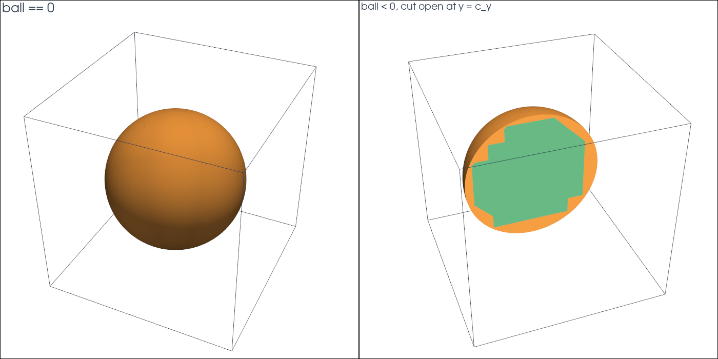
Geometry#
The background mesh covers the cube \([-1,1]^3\). The ball of radius \(R=0.7\) about \(c\) is \(B=\{x : |x-c|<R\}\), with
Implementation Order#
Build a structured tetrahedral
MeshView.Make the ball twice:
analytic_sphere, and a P2 interpolant of the same function.Cut by each and select
ball < 0andball == 0.Compare volumes and areas with the exact values.
Write curved VTU files and show the parts with PyVista.
Background Mesh#
box_mesh(..., cell_type="tetrahedron") splits every grid cube into six
tetrahedra around its diagonal. The mesh is conforming and needs only NumPy;
n = 13 points per side give 10368 tetrahedra.
mesh = cutcells.box_mesh(-1.0, -1.0, -1.0, 1.0, 1.0, 1.0, n, n, n, cell_type="tetrahedron")
For meshes from elsewhere, MeshView(coordinates, connectivity, offsets, cell_types, tdim) takes the flat arrays of any mesh of the supported cell
types, and mesh_from_pyvista converts a PyVista grid.
Exact and Interpolated Level Sets#
An analytic level set gives values, gradients and bounds of both over boxes.
cut classifies cells by the bounds, and quadrays integrates the level set
itself, with no interpolant. The interpolated ball is the P2 interpolant of
the signed distance:
exact = cutcells.analytic_sphere(CENTER, RADIUS, name="ball")
interpolated = cutcells.create_level_set(mesh, sphere, degree=2, name="ball")

for ball in (exact, interpolated):
    result = cutcells.cut(mesh, ball)
    inside = result[ball < 0]
    surface = result[ball == 0]
    volume = inside.quadrature(order=4).weights.sum()
    area = surface.quadrature(order=4).weights.sum()
Other analytic level sets come from Python callables
(cutcells.AnalyticLevelSet), from compiled geometry libraries through a
capsule, or from ShapeForest shapes; see Level sets.
Curved Output#
A part’s visualisation mesh holds Lagrange cells of the given degree: for the
sphere, curved triangles and quadrilaterals; for the ball in mode="full",
the whole tetrahedra and the curved pieces of the cut cells. Each piece knows
its background cell (parent):
inside.write_vtu("ball.vtu", mode="full", degree=3)
surface.write_vtu("sphere.vtu", mode="cut_only", degree=3)
In PyVista, extract_surface(nonlinear_subdivision=...) draws the Lagrange
cells curved:
def curved(part, subdivision=2):
    grid = cutcells.to_pyvista(part.visualization_mesh(mode="cut_only", degree=3))
    return grid.extract_surface(nonlinear_subdivision=subdivision, algorithm="dataset_surface")

plotter.add_mesh(curved(result[ball == 0]), color="#f59e42", smooth_shading=True)
To look inside the ball, cut it open with a plane given as a second level set, and draw the sphere behind the plane and the section in it. Each piece knows its background cell, which colours the section:
plane = cutcells.create_level_set(mesh, lambda X: X[1] - CENTER[1], degree=1, name="plane")
opened = cutcells.cut(mesh, [ball, plane])
shell = curved(opened[(ball == 0) & (plane < 0)])
section = curved(opened[(plane == 0) & (ball < 0)])
section.cell_data["cut"] = np.isin(section.cell_data["parent"], result.cut_cells).astype(int)
The curved cells are drawn one per piece of the quadrays decomposition, and neighbouring pieces do not share nodes: they meet up to hairline gaps, about 1e-3 wide on this mesh, which can show as specks in a close view.
Results#
background cells: 10368, cut cells: 1524
 level set   volume error   area error
     exact       1.12e-10     4.39e-08
        P2       1.38e-05     1.19e-04
With the P2 level set both errors are the interpolation error. With exact
geometry the area error at order=4 is set by the Gauss points per segment
on the curved pieces (see Convergence); with
QuadraysOptions.points_per_segment = 6 it drops to round-off.
Run the Demo#
python python/demo/demo_sphere.py
python python/demo/demo_sphere.py --n 17 --no-plot
Options: --n grid points per side, --order of the quadrature,
--output-dir for the VTU files, --no-plot and --screenshot file.png.