Degree and Order

This tutorial follows python/demo/demo_degree_order.py. A level set has a degree and a rule has an order, and each controls a different error: the degree decides which region is described, the order how well that region is integrated. The demo turns both on one ball and shows where each stops helping.

Volume and area errors against the quadrature order, for Pk level sets and the exact sphere, on 4096 hexahedra. Each curve falls until it reaches the interpolation error of its level set.

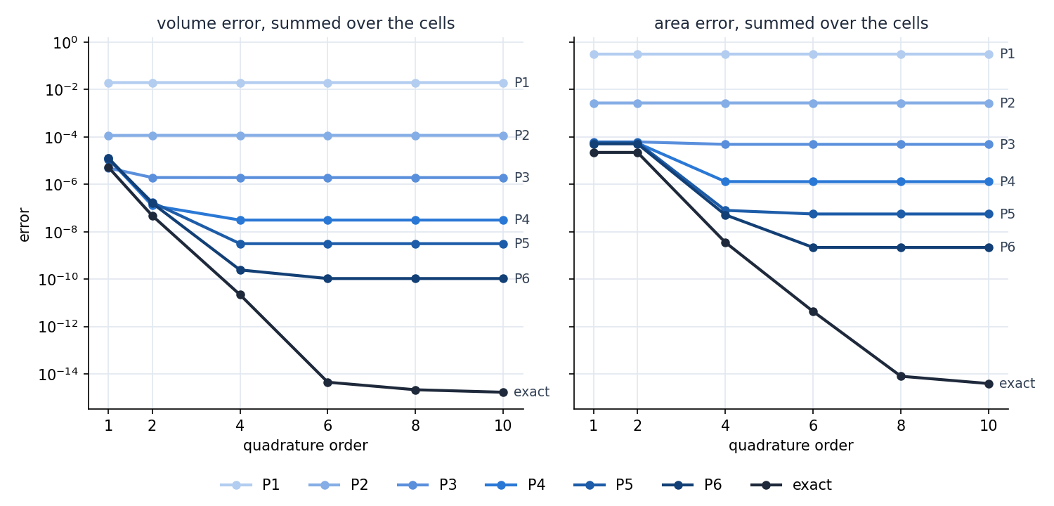
Measuring Per Cell

The ball has radius 0.6 about \((0.1, -0.05, 0.03)\), in a hexahedral mesh of \([-1, 1]^3\) with 17 grid points per side. The reference is the exact sphere integrated with 14 points per segment, cell by cell, and the error is the sum of the cells’ absolute errors:

def per_cell(rules, n_cells):
    cells = np.repeat(rules.parent_map, np.diff(rules.offset))
    return np.bincount(cells, weights=rules.weights, minlength=n_cells)

error = np.abs(per_cell(rules, n_cells) - reference).sum()

The error of the total would look far better, because neighbouring cells err by opposite amounts. For P2 at order 6 the total volume is off by 6.1e-7, while the cells are off by 1.2e-4 together. A cut finite element method assembles cell by cell, so the per-cell number is the one that matters to it.

Two Dials

phi = cutcells.create_level_set(mesh, sphere, degree=degree, name="phi")
result = cutcells.cut(mesh, phi)
volume = result[phi < 0].quadrature(order=order)
surface = result[phi == 0].quadrature(order=order)

volume error
 order        1        2        4        6        8       10
    P1  2.0e-02  2.0e-02  2.0e-02  2.0e-02  2.0e-02  2.0e-02
    P2  1.2e-04  1.2e-04  1.2e-04  1.2e-04  1.2e-04  1.2e-04
    P3  4.9e-06  1.9e-06  1.9e-06  1.9e-06  1.9e-06  1.9e-06
    P4  1.3e-05  1.3e-07  3.1e-08  3.1e-08  3.1e-08  3.1e-08
    P5  1.1e-05  1.7e-07  3.1e-09  3.1e-09  3.1e-09  3.1e-09
    P6  1.3e-05  1.6e-07  2.4e-10  1.1e-10  1.1e-10  1.1e-10
 exact  5.3e-06  4.8e-08  2.2e-11  4.5e-15  2.1e-15  1.7e-15

area error
 order        1        2        4        6        8       10
    P1  3.1e-01  3.1e-01  3.1e-01  3.1e-01  3.1e-01  3.1e-01
    P2  2.7e-03  2.7e-03  2.7e-03  2.7e-03  2.7e-03  2.7e-03
    P3  6.2e-05  6.2e-05  4.9e-05  4.9e-05  4.9e-05  4.9e-05
    P4  5.5e-05  5.5e-05  1.3e-06  1.3e-06  1.3e-06  1.3e-06
    P5  5.8e-05  5.8e-05  8.0e-08  5.6e-08  5.6e-08  5.6e-08
    P6  5.1e-05  5.1e-05  5.2e-08  2.2e-09  2.2e-09  2.2e-09
 exact  2.2e-05  2.2e-05  3.6e-09  4.3e-12  8.0e-15  3.9e-15

Read each row from the left: it falls with the order and then stays flat. The flat part is the interpolation error of the level set, which no rule can improve. Read each column from the top: at a low order all the higher degrees give about the same error, because the rule limits them.

So the two dials should be raised together. Up to P4, order 4 reaches the floor. P5 and P6 need order 6. Beyond that floor, extra order only adds points. Orders 1 and 2 give the same surface rule, as the area columns show.

What Each Dial Costs

points per cut cell, volume / surface
 order         1         2         4         6         8        10
    P1    23/7      61/7     135/19    281/37    540/52    812/76
    P2    26/9      59/9     209/32    554/59   1018/98   1616/146
    P3    35/9      63/9     193/32    542/59   1003/99   1531/144
    P4    31/10     56/10    207/32    537/64   1051/106  1537/159
    P5    33/11     58/11    195/29    458/57    889/94   1290/140
    P6    33/11     58/11    190/29    439/55    857/91   1225/136
 exact    29/8      62/8     230/33    570/62   1055/101  1658/149

The order sets the number of points. The degree does not raise it: P6 at order 6 takes fewer points than P2 at order 6, and its error is five to six orders of magnitude lower.

The degree is paid for elsewhere, in cut, which bounds each level set in its Bernstein form on every cell:

cost at order 6
        interpolate       cut  rules, us per cut cell
    P1       0.061s    0.014s                     461
    P2       0.064s    0.026s                    1287
    P3       0.107s    0.069s                    2181
    P4       0.145s    0.178s                    3142
    P5       0.319s    1.195s                    5255
    P6       0.582s    5.213s                   10825
 exact       0.000s    0.010s                    1578

The times were taken on a busy machine, so read them for their size only. cut grows by three to seven times per degree on hexahedra, faster at the higher degrees: a separate run took 4.7 s for P6 and 77 s for P8 on these 4096 hexahedra, against 1.4 s and 6.2 s on 24576 tetrahedra of the same grid. Degrees up to about 5 are the practical range on hexahedra.

When the geometry is known

The exact sphere needs no interpolation, reaches round-off at order 6 for the volume and order 8 for the area, takes as many points as P2 and has the cheapest cut. If you can write the level set down, analytic_sphere and the other C++ level sets beat any interpolant. A level set from Python callbacks gives the same volume to 11 digits but pays for every call:

analytic level sets, 512 hexahedra, order 4
     C++:    0.033 s, volume 0.904778684261
  Python:    3.757 s, volume 0.904778684262

Its box_bounds must also bound the gradient, as in the demo. With only the two bounds of the value, quadrays cannot certify a box and bisects to its limits; the same run took well over an hour and lost accuracy.

Run the Demo

python python/demo/demo_degree_order.py
python python/demo/demo_degree_order.py --n 9 --python-level-set --no-plot

Options: --n grid points per side, --python-level-set to time the callbacks, --no-plot to skip the matplotlib window and --screenshot file.png to save the plot.